Periodically I see questions or comments about how we use operations research in our personal lives. The truth, of course, is that for the most part we don't. We may use the systematic analysis and critical thinking inherent in OR, but generally we neither need nor bother with the mathematical models. (As an example of the "critical thinking", consider the ads you see on TV for insurance companies, touting that "customers who switched to <insert company name> saved an average of <insert large positive amount> on their premiums". A typical viewer may think "wow, they're pretty cheap". An OR person thinks "no kidding -- people with negative savings didn't switch, so the data is censored".) Recently, however, I actually found an application for an OR model in my personal life.
In the aftermath of the "Financial Debacle of 2008" (or the "Great Recession", or whatever you prefer to call it), banks are scrambling to make money. Thus, among other things, credit card rebate programs have become more byzantine. Once upon a time, my Chase credit card earned rebates that were simply posted monthly, automatically and in the full amount I'd earned. Couldn't have been simpler. Didn't last.
I now "enjoy" the benefits of the Chase Ultimate Rewards program. Rebates are no longer credited automatically; I have to log in each month and claim them. There can be delays in how quickly they post. Rebate balances below \$20 cannot be redeemed (they carry over to the following month). I have options for claiming the rewards, including buying things I don't need through Chase (probably at higher than market prices) or asking them to cut me a check (then waiting for it to arrive, then depositing it somewhere). The most convenient (or should I say least inconvenient?) way to redeem them may be what Chase calls the "pay yourself back" option, in which you apply the rebate to purchases made within the past 60 days. The amount redeemed shows up as a credit on your next statement.
Besides the delay in receiving the credit, there are other minor hassles with the "pay yourself back approach". You cannot pay yourself back for part of a purchase; you must have sufficient rebate credit accumulated to pay back the entire amount. The web form only allows you to pay back one purchase at a time, and the \$20 minimum limit applies to each individual redemption, not to the combined set of redemptions. Most of the time, this is a non-issue for me, since it usually takes me more than one billing cycle to accrue a rebate balance above \$20, at which point I immediately repay myself for a recent \$20+ purchase and drop the remaining balance back below \$20, to sit for another cycle or two.
Occasionally, however, some combination of unusual expenditures gets me a larger balance. The trick then is to find a collection of purchases within the past 60 days, each \$20 or more, whose combined total comes closest to my available rebate balance without exceeding it. That's probably trial-and-error for most people, but readers of this blog may recognize the problem as a binary knapsack, where the value and "size" of an item are both the amount charged, the constraint limit is the available rebate balance, and only recent purchases of \$20 or more make it into the model. So I now have a spreadsheet containing just that model, which I'll probably need once or perhaps twice a year.
Sunday, December 26, 2010
Friday, December 24, 2010
A Seasonal TSP (Traveling Santa Problem)
You can tell when academics with blogs are between semesters by the increased frequency of their postings. Yesterday Laura McLay posted a pointer to a 12-city traveling Santa problem (PDF file) at Math-Drills.Com. Faced with a Christmas Eve choice of (a) paying bills, (b) performing some overdue data analysis for a paper-to-be or (c) playing with a TSP ... well, let's just say that I didn't need the Analytic Hierarchy Process to sort that one out.
Slightly (well, very slightly) more seriously, I was curious about the difficulty of the problem. The TSP is one of the quintessential NP-hard problems, with all sorts of special purpose algorithms devised for it. Sometimes, though, I think we confuse NP-hard with hard. NP-hard refers to a class of problems. At the risk of starting a flame war with purists (which will at least drive up my site stats), all optimization problems get pretty darn hard when they're big enough; we tend to believe that NP-hard problems get pretty darn hard faster than NP-not-so-hard problems as their size grows. What is sometimes overlooked, though, is that all this is a sort of asymptotic result; we can solve not horribly large problems pretty easily (I can do the three city TSP in my head, at least after a cup or two of coffee), and the dividing line between doable and not doable continually shifts with improvements in hardware and software.
I wasn't really motivated enough to look up the latest and greatest algorithms for TSPs, so I started with an old, and I'm sure now "obsolete", method due I believe to Miller, Tucker and Zemlin ca. 1960. It's a mixed integer linear programming formulation using binary variables to determine which links are included in the Hamiltonian circuit (route). There are additional nonnegative variables that assign what we might call "potentials" to each node. We require each node to be entered and exited once, and we require that any time a link is used, the potential of the destination city be at least one greater than the potential of the origin city, unless the destination city is the starting point for the circuit (i.e., unless the link closes the loop). The MTZ formulation is more compact than formulations built with subtour elimination constraints (of which exponentially many can occur), but I believe it tends to have weaker bounds (and I've seen some papers on tightening the bounds in the MTZ formulation, but can't recall any details).
Anyway, driving back and forth between home and the YMCA (one of two loci of physical self-abuse for me), I mapped out a general strategy: write a MILP model using the MTZ approach and see how long it takes to solve (using the Java API to CPLEX 12.2); see if identifying the single entry/single exit constraints as SOS1 sets (with "cleverly chosen" weights) helps; maybe try adding cuts on the fly to eliminate dominated segments of the tour (don't go A-B-C-D if A-C-B-D is shorter); maybe try depth-first search; etc., etc. As always, to paraphrase someone (Napoleon?), the first casualty in every battle is the plan. I wrote the basic MILP model with MTZ constraints pretty quickly (copying the data out of the PDF and into the Java editor, suitably reformatted, actually took longer than writing the code itself) and turned CPLEX loose with all default settings. CPLEX found an optimal solution in something around 0.3 seconds (on my dual core laptop). So much for any experiments in parameter tweaking, SOS1, and so on.
I won't publish the optimal route here, in case anyone is still working on it, but I will say that the length of the optimal solution is 30,071 miles -- and this is only 12 of the cities Santa must visit. I hope he remembered to feed the reindeer.
Thursday, December 23, 2010
Interesting Essay on Mathematics and Education
Many thanks to Larry at IEORTools for pointing out an essay by Dr. Robert H. Lewis of Fordham University entitled "Mathematics: The Most Misunderstood Subject". It's a worthwhile read for any math geek (and, face it, if you're reading OR blogs you're probably a math geek). Besides some insightful comments about the state of mathematical education, it's a nice reminder that math is not just about answers.
Tuesday, December 21, 2010
New Toy for the Holiday: Google N-gram Viewer
Staring at one of the graphs in a recent post on the bit-player blog ("Googling the lexicon"), I was struck by a downward trend in the frequency of the phrase "catastrophe theory". That led me to do a few searches of my own on Google's n-gram viewer, which is one of those insidiously fascinating Internet gadgets that suck away so much productivity. (Who am I trying to kid? It's Christmas break; how productive was I going to be anyway??) Being a closeted mathematician, I first did a comparison of three recent "fads" (perhaps an unfair characterization) in math: catastrophe theory, chaos theory and fractal geometry.

Then I took a shot with a few terms from optimization: genetic algorithms, goal programming, integer programming and linear programming.

I find it a bit surprising that chaos theory gets so much more play than fractal geometry (which has some fairly practical applications, as Mike Trick noted in his eulogy for Benoit Mandelbrot). Two other things (one I find serendipitous, one less so) struck me about the graphs.
The serendipitous note is that references to catastrophe theory are tailing off. I recall sitting at a counter in a chain restaurant during my graduate student days, scarfing down breakfast while trying to chew my way through a journal article on catastrophe theory (which was rather new at that time). Differential equations (especially nonlinear PDEs) were not my strong suit, to put it charitably, and the article was heavy going. A few years later social scientists heard about catastrophe theory. As I recall, the canonical image for it was a trajectory for a PDE solution on a manifold that "fell off a cliff" (picture your favorite waterfall here). Social scientists are in the main clueless about differential equations (let alone PDEs on manifolds), but waterfalls they get. The next thing I knew, all sorts of political science and maybe anthropology papers (not sure about the latter) were saying "catastrophe theory this" and "catastrophe theory that", and I'm pretty sure they were abusing it rather roundly. So I interpret the decline in references as at least in part indicating it has reverted to its natural habitat, among a fairly small group of mathematicians who actually grok the math.
The less serendipitous note is that all the graphs are showing downward trends. Since the vertical axis is in percentage terms, I cannot attribute this to a reduction in the number of published books, nor blame it on the Blackberry/iPod/whatever technical revolution. My fear is that interest in mathematics in general may be on the decline. Perhaps what we need now is for the next installment of the "Harry Potter" series to have Harry defeating the Dark Lord by invoking not incantations but mathematical models (but not catastrophe theory, please).
Friday, December 17, 2010
Defining Analytics
This should probably be a tweet, except I've so far resisted the temptation to be involved with something that would associate my name with any conjugation of "twit". As noted by Mike Trick and others, "analytics" is catching on as the new buzzword for ... well, something, and likely something strongly related if not identical to operations research. So now we need a definition of "analytics". A recent article by four reasonably senior people at IBM (appropriately, in the Analytics webzine) attempts to give a fairly inclusive definition, incorporating three major categories: description; prediction; and prescription. Hopefully this, or something like it, will catch on, lest "analytics" be equated to statistical data dredging and/or the study of sheep entrails.
We're an IE Blog!
There are periodic discussions on various forums about how to define operations research, and the even trickier question of how one distinguishes operations research from management science from industrial engineering (or even if such distinctions are meaningful). So it comes as no surprise to me that the definition of "industrial engineering" may be evolving. It did come as a bit of a surprise, however, when I was notified today by Rachel Stevenson, co-founder of Engineering Masters, that this blog had made their "Top 50 Industrial Engineering Blogs" list. (Not as big a shock as when I found myself teaching organizational behavior, though, and considerably more pleasant!) I was particularly gratified by my #8 ranking ... until I realized it was alphabetical by blog title within groups.
The categories listed in the Engineering Masters blog post tell us something about the range of interests people with IE degrees might have these days. Besides operations research, they have operations management, project management, financial engineering (where the intent is to make something out of nothing and recent practice, at least, has been to make nothing out of a whole pile of something), machine learning, statistics (which I find interesting since AFAIK the average engineering major takes approximately one statistics course), analytics (another definitional debate in the making), and life-cycle management (who knew that would spawn so many blogs?).
Like any blog roll, there's a reciprocity at work here: they link my blog (and maybe drive a second reader to it), and I link their blog (and maybe drive my one current reader to it). I'm okay with that: it's free (unlike the occasional pitches I get for including me in the who's who of academic bloviators, presumably to get me to buy the book), I'm not embarrassed to point to their site, and I'm pretty sure it generates no money for terrorists, organized crime or political parties. (Apologies if those last two are redundant.) If nothing else, I appreciate their efforts compiling the list of blogs because I see a few entries on it that look promising, of which I would otherwise be unaware.
Friday, December 10, 2010
How to Avoid Choking
I have three final exams to inflict next week, so I found a recent article by Discover Magazine quite timely. It cites research by Dr. Sian Beilock of the University of Chicago (who has dual doctorates from Michigan State University, so she must know whereof she speaks!), indicating that paying too much attention to what you are doing can cause your performance to deteriorate. As a student of Tae Kwon Do and one of life's natural non-athletes, I can relate to this: it often seems that the more I try to focus on the mechanics of a technique, the worse I do it (much like a baseball pitcher who "steers" pitches).
According to the article, Dr. Beilock
According to the article, Dr. Beilock
has found that test takers, speech givers, musicians, and top athletes fail in similar ways.If this is indeed true, then shouldn't the students who pay little to no attention to what they are doing on their exams outperform their classmates? I've got more than a few of them, and by and large their inattention is not paying off for them.
Modeling the All Units Discount
In a previous entry, I discussed how to incorporate continuous piecewise linear functions in a mathematical program. There are times, however, when you have to model a discontinuous piecewise linear function. A classic example is the all units discount, where exceeding a quantity threshold (called a breakpoint) for a product order garners a reduced price on every unit in the order. (The incremental discount case where the price reduction applies only to units in excess of the breakpoint, is covered in the prior entry.) SOS2 variables, which I used in the first post, will not work here because they model a continuous function.
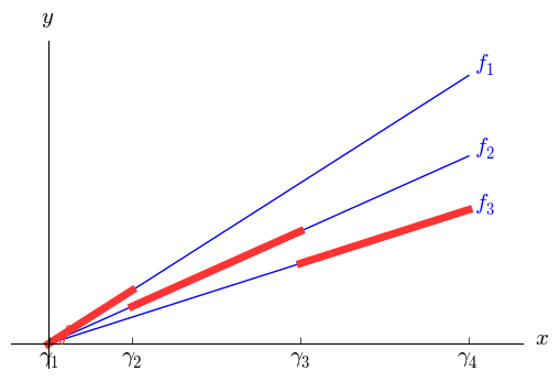
Let $y$ be a quantity (typically cost) that we wish to minimize. As before, we will assume that $y$ is a piecewise linear function of some variable $x$; for simplicity, I'll assume bounds $0 \le x \le U$ and $y\ge 0$. Let $0 = \gamma_1 < \cdots < \gamma_N < \gamma_{N+1}=U$ denote the breakpoints, and let $y=f_i(x)=\alpha_i x + \beta_i$ when $\gamma_i \le x < \gamma_{i+1}$, with the adjustment that the last interval is closed on the right ($f(U)=\alpha_N U + \beta_N$). With all units discounts, it is typical that the intercepts are all zero ($\beta_1 = \cdots = \beta_N = 0$) and cost ($y$) is proportional to volume ($x$), as seen in the first graph below, but we need not assume that. The second graph illustrates a somewhat more general case. In fact, we need not assume an economy of scale; the same modeling approach will work with a diseconomy of scale.


To model the discount, we need to know into which interval $x$ falls. Accordingly, we introduce binary variables $z_1,\ldots ,z_N$ and add the constraint $$\sum_{i=1}^N z_i = 1,$$ effectively making $\{z_1,\ldots , z_n\}$ an SOS1 set. Let $$M_i = \max_{0 \le x \le U} f_i(x)$$ for $i=1,\ldots,N$. Typically $M_i = f_i(U)$, but again we need not assume that. To connect the binary variables to $x$, we add for each $i\in \{1,\ldots,N\}$ the constraint $$\gamma_i z_i \le x \le \gamma_{i+1} z_i + U(1-z_i).$$ This just repeats the domain $0\le x \le U$ for all but the one index $i$ with $z_i = 1$; for that index, we get $\gamma_i \le x \le \gamma_{i+1}$.
The last piece is to relate the binary variables to $y$. We handle that by adding for each $i\in \{1,\ldots,N\}$ the constraint $$y\ge \alpha_i x + \beta_i - M_i(1-z_i).$$ For all but one index $i$ the right hand side reduces to $f_i(x)-M_i \le 0$. For the index $i$ corresponding to the interval containing $x$, we have $y\ge f_i(x)$. Since $y$ is being minimized, the solver will automatically set $y=f_i(x)$.
Adjustments for nonzero lower bounds for $x$ and $y$ are easy and left to the reader as an exercise. One last thing to note is that, while we can talk about semi-open intervals for $x$, in practice mathematical programs abhor regions that are not closed. If $x=\gamma_{i+1}$, then the solver has a choice between $z_i=1$ and $z_{i+1}=1$ and will choose whichever one gives the smaller value of $y$. This is consistent with typical all units discounts, where hitting a breakpoint exactly qualifies you for the lower price. If your particular problem requires that you pay the higher cost when you are sitting on a breakpoint, the model will break down. Unless you are willing to tolerate small gaps in the domain of $x$ (so that, for instance, the semi-open interval $[\gamma_i ,\gamma_{i+1})$ becomes $[\gamma_i , \gamma_{i+1}-\epsilon]$ and $x$ cannot fall in $(\gamma_{i+1}-\epsilon,\gamma_{i+1})$), you will have trouble modeling your problem.
Let $y$ be a quantity (typically cost) that we wish to minimize. As before, we will assume that $y$ is a piecewise linear function of some variable $x$; for simplicity, I'll assume bounds $0 \le x \le U$ and $y\ge 0$. Let $0 = \gamma_1 < \cdots < \gamma_N < \gamma_{N+1}=U$ denote the breakpoints, and let $y=f_i(x)=\alpha_i x + \beta_i$ when $\gamma_i \le x < \gamma_{i+1}$, with the adjustment that the last interval is closed on the right ($f(U)=\alpha_N U + \beta_N$). With all units discounts, it is typical that the intercepts are all zero ($\beta_1 = \cdots = \beta_N = 0$) and cost ($y$) is proportional to volume ($x$), as seen in the first graph below, but we need not assume that. The second graph illustrates a somewhat more general case. In fact, we need not assume an economy of scale; the same modeling approach will work with a diseconomy of scale.

To model the discount, we need to know into which interval $x$ falls. Accordingly, we introduce binary variables $z_1,\ldots ,z_N$ and add the constraint $$\sum_{i=1}^N z_i = 1,$$ effectively making $\{z_1,\ldots , z_n\}$ an SOS1 set. Let $$M_i = \max_{0 \le x \le U} f_i(x)$$ for $i=1,\ldots,N$. Typically $M_i = f_i(U)$, but again we need not assume that. To connect the binary variables to $x$, we add for each $i\in \{1,\ldots,N\}$ the constraint $$\gamma_i z_i \le x \le \gamma_{i+1} z_i + U(1-z_i).$$ This just repeats the domain $0\le x \le U$ for all but the one index $i$ with $z_i = 1$; for that index, we get $\gamma_i \le x \le \gamma_{i+1}$.
The last piece is to relate the binary variables to $y$. We handle that by adding for each $i\in \{1,\ldots,N\}$ the constraint $$y\ge \alpha_i x + \beta_i - M_i(1-z_i).$$ For all but one index $i$ the right hand side reduces to $f_i(x)-M_i \le 0$. For the index $i$ corresponding to the interval containing $x$, we have $y\ge f_i(x)$. Since $y$ is being minimized, the solver will automatically set $y=f_i(x)$.
Adjustments for nonzero lower bounds for $x$ and $y$ are easy and left to the reader as an exercise. One last thing to note is that, while we can talk about semi-open intervals for $x$, in practice mathematical programs abhor regions that are not closed. If $x=\gamma_{i+1}$, then the solver has a choice between $z_i=1$ and $z_{i+1}=1$ and will choose whichever one gives the smaller value of $y$. This is consistent with typical all units discounts, where hitting a breakpoint exactly qualifies you for the lower price. If your particular problem requires that you pay the higher cost when you are sitting on a breakpoint, the model will break down. Unless you are willing to tolerate small gaps in the domain of $x$ (so that, for instance, the semi-open interval $[\gamma_i ,\gamma_{i+1})$ becomes $[\gamma_i , \gamma_{i+1}-\epsilon]$ and $x$ cannot fall in $(\gamma_{i+1}-\epsilon,\gamma_{i+1})$), you will have trouble modeling your problem.
Wednesday, December 8, 2010
LPs and the Positive Part
A question came up recently that can be cast in the following terms. Let $x$ and $y$ be variables (or expressions), with $y$ unrestricted in sign. How do we enforce the requirement that \[
x\le y^{+}=\max(y,0)\] (i.e., $x$ is bounded by the positive part of $y$) in a linear program?
To do so, we will need to introduce a binary variable $z$, and we will need lower ($L$) and upper ($U$) bounds on the value of $y$. Since the sign of $y$ is in doubt, presumably $L<0<U$. We add the following constraints:\begin{align*} Lz & \le y\\ y & \le U(1-z)\\ x & \le y-Lz\\ x & \le U(1-z)\end{align*} Left to the reader as an exercise: $z=0$ implies that $0\le y \le U$ and $x \le y \le U$, while $z=1$ implies that $L \le y \le 0$ and $x \le 0 \le y-L$.
We are using the binary variable $z$ to select one of two portions of the feasible region. Since feasible regions in mathematical programs need to be closed, it is frequently the case that the two regions will share some portion of their boundaries, and it is worth checking that at such points (where the value of the binary variable is uncertain) the formulation holds up. In this case, the regions correspond to $y\le 0$ and $y\ge 0$, the boundary is $y=0$, and it is comforting to note that if $y=0$ then $x\le 0$ regardless of the value of $z$.
Saturday, December 4, 2010
OR and ... Parking??
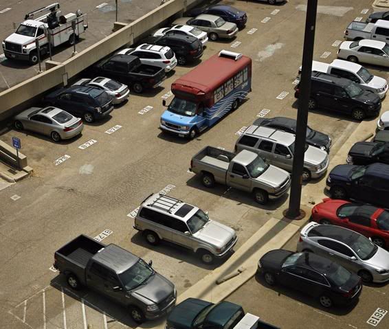
The application of stopping rules is fairly obvious, although the rule to use may not be. You're running a search pattern through the packed parking lot of a mall, looking for an empty spot, when lo and behold you find one. Now comes the stopping rule: do you grab it, or do you continue the search, hoping for one closer to your immediate destination (the first store you plan to hit)? If you pass it up and fail to find something closer, it likely will not be there the next time you go by. Add an objective function that balances your patience (or lack thereof), your tolerance for walking, the cost of fuel, any time limits on your shopping spree and the possibility of ending up in a contest for the last spot with a fellow shopper possessing less holiday spirit (and possibly better armed than you), and you have the stopping problem.
The other obvious aspect is optimization of a distance metric, and this part tends to amuse me a bit. Some people are very motivated to get the "perfect" spot, the one closest to their target. My cousin exhibits that behavior (in her defense, because walking is painful), as did a lady I previously dated (for whom it was apparently a sport). Parking lots generally are laid out in a rectilinear manner (parallel rows of spaces), and most shoppers seem to adhere rather strictly to the L1 or "taxicab" norm. That's the appropriate norm for measuring driving distance between the parking spot and the store, but the appropriate norm for measuring walking distance is something between the L1 and L2 or Euclidean norm. Euclidean norm is more relevant if either (a) the lot is largely empty or (b) you are willing to walk over (or jump over) parked cars (and can do so without expending too much additional energy). Assuming some willingness to walk between parked cars, the shortest path from most spots to the store will be a zig-zag (cutting diagonally across some empty spots and lanes) that may, depending on circumstances, be closer to a geodesic in the taxicab geometry (favoring L1) or closer to a straight line (favoring L2). The upshot of this is that while some drivers spend considerable time looking for the L1-optimal spot (and often waiting for the current occupant to surrender it), I can frequently find a spot further away in L1 but closer in L2 and get to the store faster and with less (or at least not much more) walking.
This leaves me with two concluding thoughts. The first is that drivers may be handicapped by a failure to absorb basic geometry (specifically, that the set of spots at a certain Euclidean distance from the store will be a circular arc, not those in a certain row or column of the lot). Since it was recently reported that bees can solve traveling salesman problems (which are much harder), I am forced to conclude that bees have a better educational system than we do, at least when it comes to math. The second is that, given the obesity epidemic in the U.S., perhaps we should spend more time teaching algorithms for the longest path problem and less time on algorithms for the shortest path problem.
[Confession: This post was motivated by the INFORMS December Blog Challenge -- because I thought there should be at least one post that did not involve pictures of food!]
Wednesday, November 24, 2010
Conference (snore) Presentations
The annual meeting of the Decision Sciences Institute just wrapped up in normally warm-and-sunny San Diego (which was neither this week). I achieved the dubious first of having to attend three committee meetings in two consecutive time slots (which means I "session-hopped" committee meetings). Let's see ... I left Lansing MI for cool, rainy weather and committee meetings ... remind me again why. Two conferences in three weeks is a bit draining, and knowing I'm going home to grading doesn't improve my disposition.
So I'm in the proper frame of mind to make the following observations about conference presentations and sessions, in no particular order:
So I'm in the proper frame of mind to make the following observations about conference presentations and sessions, in no particular order:
- Assume that your audience is reasonably smart. Don't explain the obvious. If you're presenting a scheduling model for buses, don't spend time explaining to the audience what a bus is. (That's not exactly what one presenter did, but it's very close.) If your audience is really that clueless, they won't understand your presentation anyway (and quite likely they're in the wrong room).
- Session chairs should enforce time limits ruthlessly. If people want to discuss the paper with the author and the author has exhausted his/her time allocation, they can do so after the session. Besides facilitating session hopping (the least important reason for this, in my opinion), it provides an incentive for authors to shorten their presentations. Also (and this is frequently overlooked), it's harder for the next presenter to gauge how much time they have left when they start at an off-cycle time in a session that's already behind schedule.
- The DSI meeting was plagued by no-show presenters (including one session where I went only to hear one paper -- the one that ended up not being presented). Occasionally a presenter is missing due to illness or death in the family (the latter happened to me once at a conference). Sometimes their funding falls through at the last minute. More often they just wanted to get in the proceedings, or they saw they were scheduled for the rump session and decided not to bother. I'm generally inclined to believe that a no-show presenter actually did the audience a favor: if they weren't committed to showing up, how committed were they to doing a good job preparing the presentation?
- As a presenter, less is more. (And I confess to screwing this one up myself at the Austin INFORMS meeting.) Leave time for feedback. Other than the minor value of another line on your vita and the major value of qualifying you for travel funds, the main virtue of presenting a paper is to get feedback from the audience. Dazzling them with your brilliance is beside the point, since the (presumed) future publication in a (presumed) top-tier journal will accomplish that.
- Graphs are good; tables of numbers are not. Tables of numbers in 4 point font (because that's what it took to fit all the numbers on one slide) are even less useful (other than to audience members who have not been sleeping well at their hotels).
- If your slides include any complete paragraphs (other than memorable quotations), say goodbye to your audience. They'll be off catching up on e-mails. If you are reading those complete paragraphs to your audience, they'll be busy e-mailing they sympathies to your students (who presumably suffer the same fate, but more regularly).
Wednesday, November 17, 2010
Obscure Engineering Conversion Factors
The following came around in this morning's e-mail, and I think it's amusing enough to be worth archiving. I've enlisted the aid of the Wikipedia to explain some of the jokes that rely on immersion in American culture.
- Ratio of an igloo's circumference to its diameter = Eskimo Pi
- 2000 pounds of Chinese Soup = Won ton
- 1 millionth of a mouthwash = 1 microscope
- Time between slipping on a peel and smacking the pavement = 1bananosecond
- Weight an evangelist carries with God = 1 billigram
- Time it takes to sail 220 yards at 1 nautical mile per hour = Knotfurlong
- 365.25 days of drinking low calorie beer = 1 Lite year
- 16.5 feet in the Twilight Zone = 1 Rod Serling
- Half a large intestine = 1 semicolon
- 1,000,000 aches = 1 megahurtz
- Basic unit of laryngitis = 1 hoarsepower
- Shortest distance between two jokes = a straight line
- 453.6 graham crackers = 1 pound cake
- 1 million microphones = 1 megaphone
- 1 million bicycles = 1 megacycle
- 365 bicycles = 1 unicycle
- 2000 mockingbirds = two kilomockingbirds
- 10 cards = 1 decacard
- 52 cards = 1 deckacard
- 1 kilogram of falling figs = 1 Fig Newton
- 1000 ccs of wet socks = 1 literhosen
- 1 millionth of a fish = 1 microfiche
- 1 trillion pins = 1 terrapin
- 10 rations = 1 decaration
- 100 rations = 1 C-Ration
- 2 monograms = 1 diagram
- 8 nickels = 2 paradigms
- 5 statute miles of intravenous surgical tubing at Yale University Hospital = 1 I.V. League
Hidden Assumptions, Unintended Consequences
The New York Times has an amusing "Budget Puzzle" that allows you to select various options for budget cuts and tax increases at the federal level, in an attempt to close the anticipated US federal deficits for 2015 and 2030. The visible math is basic addition and subtraction, but hidden below the projected results of each option are various unstated assumptions. Many of these assumptions will be economic in nature, and economists have been known to make some entertaining assumptions. (Do you remember that bit in Econ 101 about the ideal production level for a firm being the quantity where marginal cost equals marginal revenue? Do you recall any mention of a capacity limit?)
Also missing from the NYT puzzle are projections of indirect costs for any of the options. If we reduce our military presence in Afghanistan drastically, will we subsequently need to make an expensive redeployment there? If we increase taxes on employer-paid health care policies, will employers reduce the availability of those policies and, if so, will that indirectly impose greater health care costs on the federal government?
It's obvious why the Times puzzle does not go into those considerations -- they're involve considerable uncertainty, and they would probably make the puzzle too complicated to be entertaining. As OR people, we're used to making assumptions (frequently designed to simplify a real-world mess into a tractable problem); but we should also be acutely aware that the puzzle contains many unstated assumptions, and not attach too much credibility to the results.
Incidentally, I balanced the budget with 34% spending cuts and 66% tax increases, and I consider myself to be a fiscal conservative (but a realist, at least in the relative topology of mathematicians).
Sunday, November 14, 2010
INFORMS Debrief
The national INFORMS meeting in Austin is in the rear-view mirror now (and I'm staring at the DSI meeting in San Diego next week -- no rest for the wicked!), so like most of the other bloggers there I feel obligated to make some (in my case random) observations about it. In no specific order ...
Enough about the conference, at least for now. It was interesting, I enjoyed interacting with some people I otherwise only see online, and I brought home a bunch of notes I'll need to sort through. I'm looking forward to next year's meeting.
- The session chaired by Laura McLay on social networking was pretty interesting, particularly as we got an extra guest panelist (Mike Trick joined Anna Nagurney, Aurelie Thiele and Wayne Winston, along with Laura) at no extra charge. Arguably the most interesting thing from my perspective was the unstated assumption that those of us with blogs would actually have something insightful to say. I generally don't, which is one reason I hesitated for a long time about starting a blog.
- On the subject of blogs, shout-out to Bjarni Kristjansson of Maximal Software, who more or less badgered me into writing one at last year's meeting. Bjarni, be careful what you wish for! :-) It took me some digging to find Bjarni's blog (or at least one of them). Now if only I could read Icelandic ...
- I got to meet a few familiar names (Tallys Yunes, Samik Raychaudhuri ) from OR-Exchange and the blogosphere.
- Thanks to those (including some above) who've added my blog to their blogrolls. The number of OR-related blogs is growing pretty quickly, but with growth come scaling issues. In particular, I wonder if we should be looking for a way to provide guidance to potential readers who might be overwhelmed with the number of blogs to consider. I randomly sample some as I come across them, but if I don't see anything that piques my interest in a couple or so posts I'm liable to forget them and move on, and perhaps I'm missing something valuable. This blog, for instance, is mostly quantitative (math programming) stuff, but with an occasional rant or fluff piece (such as this entry). I wonder if we could somehow publish a master blog roll with an associated tag cloud for each blog, to help clarify which blogs contain which sorts of content.
- A consistent bug up my butt about INFORMS meetings is their use of time. Specifically, the A sessions run 0800 to 0930, followed by coffee from 0930 to 1000. There is then an hour that seems to be underutilized (although I think some plenaries and other special sessions occur then -- I'm not sure, as I'm not big on attending plenary talks). The B sessions run 1100 to 1230 and the C sessions run 1330 to 1500. So we have an hour of what my OM colleagues call "inserted slack" after the first coffee break, but only one hour to get out of the convention center, find some lunch and get back. It would be nice if the inserted slack and the B session could be flipped, allowing more time for lunch. My guess is that the current schedule exists either to funnel people into plenaries (who might otherwise opt for an extended lunch break) or to funnel them into the exhibits (or both).
- We're a large meeting, so we usually need to be in a conference center (the D.C. meeting being an exception). That means we're usually in a business district, where restaurants that rely on office workers for patronage often close on Sundays (D.C. and San Diego again being exceptions). Those restaurants that are open on Sunday seem to be caught by surprise when thousands of starving geeks descend en masse, pretty much all with a 1230 - 1330 lunch hour. For a society that embraces predictive analytics, we're not doing a very good job of communicating those predictions to the local restaurants. (Could INFORMS maybe hire a wiener wagon for Sundays?)
- The layout of the Austin convention center struck me as a bit screwy even without the construction. For non-attendees, to get from the third floor to the fourth floor you had to take an escalator to the first floor (sidebar: the escalator did not stop at the second floor), walk most of the length of the facility, go outside and walk the rest of the length, go back inside and take an escalator to the fourth floor (sidebar: this escalator did not stop at either of the two intervening floors). Someone missed an opportunity to apply the Floyd-Warshall algorithm and embed shortest routes between all nodes in the map we got.
- The sessions I attended ranged from fairly interesting to very interesting, so I have absolutely no complaints about that. I also had good luck networking with people I wanted to see while I was there. Since sessions and networking are my two main reasons for attending a conference (my own presentation ranks a distant third), it was well worth the trip.
- A geek in motion will come to rest at the location that maximizes interdiction of other traffic (particularly purposeful traffic).
- A geek at rest will remain at rest until someone bearing a cup of coffee enters their detection range, at which point they will sharply accelerate on an optimized collision course.
- A geek entering or exiting a session in progress will allow the door to slam shut behind them with probability approaching 1.0. (Since I have no empirical evidence that geeks are hard of hearing, I attribute this to a very shallow learning curve for things outside the geek's immediate discipline, but I'm having trouble collecting sufficiently specific data to test that hypothesis.)
Enough about the conference, at least for now. It was interesting, I enjoyed interacting with some people I otherwise only see online, and I brought home a bunch of notes I'll need to sort through. I'm looking forward to next year's meeting.
Thursday, November 11, 2010
Metcalfe's and Clancy's Laws
I don't have a Twitter account (years of dealing with administrators have left me averse to anything with "twit" in it), so I'll blog this instead. (In any case, I couldn't do this in 140 characters. As a professor, I can't do anything in 140 words, let alone 140 characters.) Yesterday Laura McLay blogged about OR and the intelligence community, and mentioned in particular J. M. Steele's paper in Management Science titled “Models for Managing Secrets”. Steele apparently presents an argument supporting the "Tom Clancy Theorem, which states that the time to detect a secret is inversely proportional
to the square of the people that know it (stated without proof in the
Hunt for Red October)" (quoting Laura).
The people who know the secret form, at least loosely, a social network. That brings me to Metcalfe's Law, which originally stated that the value of a communications network is proportional to the square of the number of connected devices, but which has since been generalized (bastardized?) to refer to humans as well as, or rather than, devices and to cover social networks as well as communications networks. I imagine Robert Metcalfe intended value to mean value to the aggregate set of owners of the attached devices (which in his mind might well have been one organization, since he's a pioneer in local area networks), but in a social networking context we can think of value as either or both of value to the members of the network (e.g., you and your Facebook friends) or value to the owners of the underlying support structure (e.g., the owners of Facebook.com).
So, letting $T$ be the time to detect a secret, $N$ the number of people who know the secret and $V$ the value of the social network to its members (which presumably includes the originator of the secret), we have $$T=\frac{k_1}{N^2}$$ and $$V=k_2\times N^2,$$ from which we infer $$T=\frac{k_1\times k_2}{V}.$$ Since the value of the social network to the "enemy" is inversely proportional to the time required to reveal the secret, we have direct proportionality between the value of the social network to the entity trying to conceal the secret and the value of that same network to the enemies of that entity.
So now I'm off to cancel my Facebook and LinkedIn accounts. :-)
Wednesday, November 10, 2010
Continuous Knapsack with Count Constraint
A question recently posted to sci.op-research offered me a welcome respite from some tedious work that I’d rather not think about and you’d rather not hear about. We know that the greedy heuristic solves the continuous knapsack problem
to optimality. (The proof, using duality theory, is quite easy.) Suppose that we add what I’ll call a count constraint, yielding
where
. Can it be solved by something other than the simplex method, such as a variant of the greedy heuristic?
The answer is yes, although I’m not at all sure that what I came up with is any easier to program or more efficient than the simplex method. Personally, I would link to a library with a linear programming solver and use simplex, but it was amusing to find an alternative even if the alternative may not be an improvement over simplex.
The method I’ll present relies on duality, specifically a well known result that if a feasible solution to a linear program and a feasible solution to its dual satisfy the complementary slackness condition, then both are optimal in their respective problems. I will denote the dual variables for the knapsack and count constraints
and
respectively. Note that
but
is unrestricted in sign. Essentially the same method stated below would work with an inequality count constraint (
), and would in fact be slightly easier, since we would know a priori the sign of
(nonnegative). The poster of the original question specified an equality count constraint, so that’s what I’ll use. There are also dual variables (
) for the upper bounds. The dual problem is
This being a blog post and not a dissertation, I’ll assume that (2) is feasible, that all parameters are strictly positive, and that the optimal solution is unique and not degenerate. Uniqueness and degeneracy will not cause invalidate the algorithm, but they would complicate the presentation. In an optimal basic feasible solution to (2), there will be either one or two basic variables — one if the knapsack constraint is nonbinding, two if it is binding — with every other variable nonbasic at either its lower or upper bound. Suppose that
is an optimal solution to the dual of (2). The reduced cost of any variable
is
. If the knapsack constraint is nonbinding, then
and the optimal solution is
If the knapsack constraint is binding, there will be two items (
,
) whose variables are basic, with
. (By assuming away degeneracy, I’ve assumed away the possibility of the slack variable in the knapsack constraint being basic with value 0). Set
and let
and
. The two basic variables are given by
The algorithm will proceed in two stages, first looking for a solution with the knapsack nonbinding (one basic
variable) and then looking for a solution with the knapsack binding (two basic
variables). Note that the first time we find feasible primal and dual solutions obeying complementary slackness, both must be optimal, so we are done. Also note that, given any
and any
, we can complete it to obtain a feasible solution to (3) by setting
. So we will always be dealing with a feasible dual solution, and the algorithm will construct primal solutions that satisfy complementary slackness. The stopping criterion therefore reduces to the constructed primal solution being feasible.
For the first phase, we sort the variables so that
. Since
and there is a single basic variable (
), whose reduced cost must be zero, obviously
. That means the reduced cost
of
is nonnegative for
and nonpositive for
. If the solution given by (3) is feasible — that is, if
and
— we are done. Moreover, if the right side of either constraint is exceeded, we need to reduce the collection of variables at their upper bound, so we need only consider cases of
for
; if, on the other hand, we fall short of
units, we need only consider cases of
for
. Thus we can use a bisection search to complete this phase. If we assume a large value of
, the initial sort can be done in O(
) time and the remainder of the phase requires
iterations, each of which uses
time.
Unfortunately, I don’t see a way to apply the bisection search to the second phase, in which we look for solutions where the knapsack constraint is binding and
. We will again search on the value of
, but this time monotonically. First apply the greedy heuristic to problem (1), retaining the knapsack constraint but ignoring the count constraint. If the solutions happens by chance to satisfy the count constraint, we are done. In most cases, though, the count constraint will be violated. If the count exceeds
, then we can deduce that the optimal value of
in (4) is positive; if the count falls short of
, the optimal value of
is negative. We start the second phase with
and move in the direction of the optimal value.
Since the greedy heuristic sorts items so that
, and since we are starting with
, our current sort order has
. We will preserve that ordering (resorting as needed) as we search for the optimal value of
. To avoid confusion (I hope), let me assume that the optimal value of
is positive, so that we will be increasing
as we go. We are looking for values of
where two of the
variables are basic, which means two have reduced cost 0. Suppose that occurs for
and
; then
It is easy to show (left to the reader as an exercise) that if
for the current value of
, then the next higher (lower) value of
which creates a tie in (7) must involve consecutive a consecutive pair of items (
). Moreover, again waving off degeneracy (in this case meaning more than two items with reduced cost 0), if we nudge
slightly beyond the value at which items
and
have reduced cost 0, the only change to the sort order is that items
and
swap places. No further movement in that direction will cause
and
to tie again, but of course either of them may end up tied with their new neighbor down the road.
The second phase, starting from
, proceeds as follows. For each pair
compute the value
of
at which
; replace that value with
if it is less than the current value of
(indicating the tie occurs in the wrong direction). Update
to
, compute
from (7), and compute
from (5) and (6). If
is primal feasible (which reduces to
and
), stop:
is optimal. Otherwise swap
and
in the sort order, set
(the reindexed items
and
will not tie again) and recompute
and
(no other
are affected by the swap).
If the first phase did not find an optimum (and if the greedy heuristic at the start of the second phase did not get lucky), the second phase must terminate with an optimum before it runs out of values of
to check (all
). Degeneracy can be handled either with a little extra effort in coding (for instance, checking multiple combinations of
and
in the second phase when three-way or higher ties occur) or by making small perturbations to break the degeneracy.
Saturday, October 23, 2010
Change to Math Rendering
I just got done switching the handling of mathematical notation in the blog from LaTeXMathML to MathJax. I think it may be a bit easier for me to use as an author, and the fonts seem to render faster in Firefox. The main reason for the switch, though, is that statistics Google compiled on my site visitors showed 69% of viewers using Windows but only 25% using Internet Explorer. I'd like to interpret that as a sign that readers of this blog have above average intelligence (or at least common sense), but it occurred to me that the fact that IE users needed a plug-in to see the mathematical notation in some posts might have been a deterrent. Not wanting to scare anyone away, I switched to MathJax, which I believe will work on a copy of IE that lacks the plug-in (and thus cannot display MathML natively) by switching to web-based fonts automatically. I'm writing this in Firefox (on a Mint laptop that lacks a copy of IE), so testing will have to wait until my next foray in Windows.
Friday, October 22, 2010
Backing Up My Blog
I just spent an hour or so searching for options to print Blogger entries (printing just the blog entry itself, not all the widgets and other clutter) and/or back up the content. Ideally, I'd hoped to add a "print this" widget, but apparently none exists, and the best solution I found (which involved adding custom code to the template) didn't work for me because I couldn't figure out the right IDs to use for the bits I wanted to make vanish. There's still the browser print feature, but that gets you all sorts of things you probably don't want.
On the backup issue, I had better luck. There are various options for (essentially) spidering the site and storing pages, including the ScrapBook extension for Firefox (which I already use for other purposes). In my case, I found a simpler option. The key is that I already have source documents for any images I use (because I have to create them myself). For lengthier posts, particularly those with lots of math, I sometimes compose the post in LyX and transfer it to Blogger, which means the LyX document serves as a backup. So my main need is to back up just the text itself (with or without all the extra clutter), primarily for the posts that I create directly in Blogger's editor (such as this one).
Enter the DownThemAll! extension for Firefox. Once you've installed it, the process is pretty simple:
If there's a better way to do this (and particularly if there's a simply way to print just what's in the actual post), I'd love to hear it.
On the backup issue, I had better luck. There are various options for (essentially) spidering the site and storing pages, including the ScrapBook extension for Firefox (which I already use for other purposes). In my case, I found a simpler option. The key is that I already have source documents for any images I use (because I have to create them myself). For lengthier posts, particularly those with lots of math, I sometimes compose the post in LyX and transfer it to Blogger, which means the LyX document serves as a backup. So my main need is to back up just the text itself (with or without all the extra clutter), primarily for the posts that I create directly in Blogger's editor (such as this one).
Enter the DownThemAll! extension for Firefox. Once you've installed it, the process is pretty simple:
- In the Blogger dashboard, select Posting > Edit Posts and list all your posts (or all your recent posts if you've backed up the older ones). There's a limit of something like 300 posts on any one page, so if you're very prolific, you'll need to iterate a few times. (Then again, if you're that prolific, you obviously have no shortage of idle time.)
- While staring at the list of your posts (each post title being a link to view the corresponding entry), click Tools > DownThemAll! Tools > DownThemAll! in Firefox to open the a dialog in which you can select the files to download. Highlight the ones that say "View" in the description field. A quick filter on "*.html" selects them all without (so far at least) grabbing anything else.
- Select where to save them, futz with other settings if you wish, then click Start! and watch DownThemAll! suck down all your postings.
If there's a better way to do this (and particularly if there's a simply way to print just what's in the actual post), I'd love to hear it.
Tuesday, October 19, 2010
Piecewise-linear Functions in Math Programs
How to handle a piecewise-linear function of one variable in an optimization
model depends to a large extent on whether it represents an economy
of scale, a diseconomy of scale, or neither. The concepts apply generally,
but in this post I'll stick to cost functions (where smaller is better,
unless you are the federal government) for examples; application to
things like productivity measures (where more is better) requires
some obvious and straightforward adjustments. Also, I'll stick to
continuous functions today.
Let's start with a diseconomy of scale. On the cost side, this is something that grows progressively more expensive at the margin as the argument increases. Wage-based labor is a good example (where, say, time-and-a-half overtime kicks in beyond some point, and double-time beyond some other point). A general representation for such a function is \[f(x)=a_{i}+b_{i}x\mbox{ for }x\in[d_{i-1},d_{i}],\: i\in\{1,\ldots,N\}\] where $d_{0}=-\infty$ and $d_{N}=+\infty$ are allowed and where the following conditions must be met: \begin{eqnarray*}d_{i-1} & < & d_{i}\:\forall i\in\{1,\ldots,N\}\\b_{i-1} & < & b_{i}\:\forall i\in\{2,\ldots,N\}\\a_{i-1}+b_{i-1}d_{i-1} & = & a_{i}+b_{i}d_{i-1}\:\forall i\in\{2,\ldots,N\}.\end{eqnarray*}The first condition just enforces consistent indexing of the intervals, the second condition enforces the diseconomy of scale, and the last condition enforces continuity. The diseconomy of scale ensures that $f$ is a convex function, as illustrated in the following graph.
 Letting $f_{i}(x)=a_{i}+b_{i}x$, we can see from the graph that $f$ is just the upper envelope of the set of functions $\{f_{1},\ldots,f_{N}\}$ (easily verified algebraically). To incorporate $f(x)$ in a mathematical program, we introduce a new variable $z$ to act as a surrogate for $f(x)$, and add the constraints\[z\ge a_{i}+b_{i}x\;\forall i\in\{1,\ldots,N\}\] to the model. Anywhere we would use $f(x)$, we use $z$ instead. Typically $f(x)$ is either directly minimized in the objective or indirectly minimized (due to its influence on other objective terms),
and so the optimal solution will contain the minimum possible value of $z$ consistent with the added constraints. In other words, one of the constraints defining $z$ will be binding. On rare occasions this will not hold (for instance, cost is relevant only in satisfying a budget, and the budget limit is quite liberal). In such circumstances, the optimal solution may have $z>f(x)$, but that will not cause an incorrect choice of $x$, and the value of $z$ can be manually adjusted to $f(x)$ after the fact.
Now let's consider an economy of scale, such as might occur when $x$ is a quantity of materials purchases, $f(x)$ is the total purchase cost, and the vendor offers discounts for larger purchases. The marginal rate of change of $f$ is now nonincreasing as a function of $x$, and as a result $f$ is concave, as in the next graph.
 Now $f$ is the lower envelope of $\{f_{1},\ldots,f_{N}\}$. We define the segments as before, save with the middle condition reversed to $b_{i-1}>b_{i}\:\forall i\in\{2,\dots,N\}$. We cannot simply add constraints of the form \[z\le a_{i}+b_{i}x\] if we are (directly or indirectly) minimizing $z$, since $z=-\infty$ would be optimal (or, if we asserted a finite lower bound for $z$, the lower bound would automatically be optimal). In the presence of an economy of scale, we are forced to add binary variables to the formulation, either directly or indirectly. The easiest way to do this is to use a type 2 specially ordered set (SOS2) constraint, provided that the solver (and any modeling language/system) understand SOS2, and provided that $d_{0}$ and $d_{N}$ are finite. Introduce new (continuous) variables $\lambda_{0},\ldots,\lambda_{N}\ge0$ along with $z$, and introduce the following constraints:\begin{eqnarray*}\lambda_{0}+\cdots+\lambda_{N} & = & 1 \\ \lambda_{0}d_{0}+\cdots+\lambda_{N}d_{N} & = & x\\ \lambda_{0}f(d_{0})+\cdots+\lambda_{N}f(d_{N}) & = & z.\end{eqnarray*} Also communicate to the solver that $\{\lambda_{0},\ldots,\lambda_{N}\}$ is an SOS2 set. The SOS2 constraint says that at most two of the $\lambda$ variables can be nonzero, and that if two are nonzero they must be consecutive. Suppose that $\lambda_{i}$ and $\lambda_{i+1}$ are positive and all others are zero. Then the new constraints express $x$ as a convex combination of $d_{i}$ and $d_{i+1}$ (with weights $\lambda_{i}$ and $\lambda_{i+1}=1-\lambda_{i}$), and express $z=f(x)$ as a convex combination of $f(d_{i})$ and $f(d_{i+1}$) using the same weights.
If SOS2 constraints are not an option, then binary variables have to be added explicitly. Let $\delta_{i}\in\{0,1\}$ designate whether $x$ belongs to the interval $[d_{i-1},d_{i}]$ ($\delta_{i}=1$) or not ($\delta_{i}=0$). Add the following constraints:\begin{eqnarray*}\delta_{1}+\cdots+\delta_{N} & = & 1\\ x & \le & d_{i}+M(1-\delta_{i})\:\forall i\in\{1,\ldots,N\}\\ x & \ge & d_{i-1}-M(1-\delta_{i})\:\forall i\in\{1,\ldots,N\}\\ z & \ge & a_{i}+b_{i}x-M(1-\delta_{i})\:\forall i\in\{1,\ldots,N\}\end{eqnarray*} where $M$ is a suitably large constant. (This formulation will again require that $d_{0}$ and $d_{N}$ be finite.) The first constraint says that $x$ must belong to exactly one interval. If $\delta_{j}=1$, the second and third constraints force $d_{j-1}\le x\le d_{j}$ and are vacuous for all $i\neq j$ (assuming $M$ is correctly chosen). The final constraint forces $z\ge f_{j}(x)$ and is again vacuous for all $i\neq j$. Since $z$ represents something to be minimized, as before we expect $z=f_{j}(x)$ in almost all cases, and can manually adjust it in the few instances were the optimal solution contains padding.
Let's start with a diseconomy of scale. On the cost side, this is something that grows progressively more expensive at the margin as the argument increases. Wage-based labor is a good example (where, say, time-and-a-half overtime kicks in beyond some point, and double-time beyond some other point). A general representation for such a function is \[f(x)=a_{i}+b_{i}x\mbox{ for }x\in[d_{i-1},d_{i}],\: i\in\{1,\ldots,N\}\] where $d_{0}=-\infty$ and $d_{N}=+\infty$ are allowed and where the following conditions must be met: \begin{eqnarray*}d_{i-1} & < & d_{i}\:\forall i\in\{1,\ldots,N\}\\b_{i-1} & < & b_{i}\:\forall i\in\{2,\ldots,N\}\\a_{i-1}+b_{i-1}d_{i-1} & = & a_{i}+b_{i}d_{i-1}\:\forall i\in\{2,\ldots,N\}.\end{eqnarray*}The first condition just enforces consistent indexing of the intervals, the second condition enforces the diseconomy of scale, and the last condition enforces continuity. The diseconomy of scale ensures that $f$ is a convex function, as illustrated in the following graph.
and so the optimal solution will contain the minimum possible value of $z$ consistent with the added constraints. In other words, one of the constraints defining $z$ will be binding. On rare occasions this will not hold (for instance, cost is relevant only in satisfying a budget, and the budget limit is quite liberal). In such circumstances, the optimal solution may have $z>f(x)$, but that will not cause an incorrect choice of $x$, and the value of $z$ can be manually adjusted to $f(x)$ after the fact.
Now let's consider an economy of scale, such as might occur when $x$ is a quantity of materials purchases, $f(x)$ is the total purchase cost, and the vendor offers discounts for larger purchases. The marginal rate of change of $f$ is now nonincreasing as a function of $x$, and as a result $f$ is concave, as in the next graph.

If SOS2 constraints are not an option, then binary variables have to be added explicitly. Let $\delta_{i}\in\{0,1\}$ designate whether $x$ belongs to the interval $[d_{i-1},d_{i}]$ ($\delta_{i}=1$) or not ($\delta_{i}=0$). Add the following constraints:\begin{eqnarray*}\delta_{1}+\cdots+\delta_{N} & = & 1\\ x & \le & d_{i}+M(1-\delta_{i})\:\forall i\in\{1,\ldots,N\}\\ x & \ge & d_{i-1}-M(1-\delta_{i})\:\forall i\in\{1,\ldots,N\}\\ z & \ge & a_{i}+b_{i}x-M(1-\delta_{i})\:\forall i\in\{1,\ldots,N\}\end{eqnarray*} where $M$ is a suitably large constant. (This formulation will again require that $d_{0}$ and $d_{N}$ be finite.) The first constraint says that $x$ must belong to exactly one interval. If $\delta_{j}=1$, the second and third constraints force $d_{j-1}\le x\le d_{j}$ and are vacuous for all $i\neq j$ (assuming $M$ is correctly chosen). The final constraint forces $z\ge f_{j}(x)$ and is again vacuous for all $i\neq j$. Since $z$ represents something to be minimized, as before we expect $z=f_{j}(x)$ in almost all cases, and can manually adjust it in the few instances were the optimal solution contains padding.
Saturday, October 9, 2010
Binary Variables and Quadratic Terms
Generally speaking, if $x$ and $y$ are variables in a mathematical program, and you want to deal with their product $z=x y$, you will end up having a quadratic problem (which may create problems with convexity if the quadratic terms appear in constraints). There is a special case, though, when at least one of $x$ and $y$ is binary, and when the other variable is bounded. Under those assumptions, the product can be linearized.
Let $x$ be binary and let $L\le y \le U$ where $L$ and $U$ are bounds known in advance. Introduce a new variable $z$. (Programming note: Regardless of whether $y$ is real-valued, integer-valued or binary, $z$ can be treated as real-valued.) Add the following four constraints: \begin{eqnarray*} z & \le & Ux \\ z & \ge & Lx \\ z & \le & y - L(1-x) \\ z & \ge & y - U(1-x). \end{eqnarray*}
Consider first the case $x=0$, which means the product $z = x y$ should be $0$. The first pair of inequalities says $0 \le z \le 0$, forcing $z=0$. The second pair of inequalities says $y-U \le z \le y - L$, and $z=0$ satisfies those inequalities.
Now consider the case $x=1$, so that the product should be $z = y$. The first pair of inequalities becomes $L \le z \le U$, which is satisfied by $z = y$. The second pair says $y \le z \le y$, forcing $z= y$ as desired.
Wednesday, September 22, 2010
Internal model v. LP file v. SAV file
Here's a topic that arises repeatedly on the CPLEX support forums: the differences between an LP/MIP model built "internally" using CPLEX Concert technology, the same model written to a file using CPLEX's SAV format (and then read back in, or solved using the interactive solver), and the same model written to a file using CPLEX's industry-not-quite-standard LP format. Since I can never find links to previous discussions when I need them, I'll put a quick summary here. I suspect it applies to other solvers that support both binary and text file formats; I know it applies to CPLEX.
Many factors influence the sequence of pivots a solver does on an LP model and the sequence of nodes it grinds through in a MIP model. If you solve the same model two different ways, using the same or different software, you should end up with the same optimal objective value (to within rounding); that's the definition of "optimal". If you don't, either you've found a bug in the software or, more likely, your problem is mathematically ill-conditioned. Even if the problem is well-conditioned, and you get the same objective value both places, you may not get the same optimal solution. You should if the solution is unique; but if there are multiple optima, you may get one optimal solution one time and a different one the next time.
This is true even if you use the same program (for instance, CPLEX) both times. Small, seemingly innocuous things such as the order in which variable or constraints are entered, or the compiler used to compile the respective CPLEX versions, can make a difference. (Different C/C++ compilers may have different floating point algorithms encoded.)
The bigger (to me) issue, though, is that if you dump the model to a file and solve the file with the interactive solver, you are not solving the same model. You are solving what is hopefully a close (enough) replicate of the original model. The binary output format (SAV for CPLEX) will generally be closer to the original model than the text (LP or MPS for CPLEX) format will be. I'm not an expert on SAV file format, so I'll say that it is possible the SAV file is an exact duplicate. That requires not only full fidelity in representation of coefficients but also that the internal model you get by reading and processing the SAV file has all variables and constraints specified in exactly the same order that they appeared in the internal model from which the SAV file was created. I'm not sure that's true, but I'm not sure it isn't.
What I am sure of is that the text version is not in general a full-fidelity copy. Not only do we have the same questions about preservation of order, but we have the rounding problems incurred by converting a double precision binary number to a text representation and then back to a double precision binary value. If your model is well-conditioned, hopefully the differences are small enough not to affect the optimal solution. It may still affect the solution process. Suppose that you have an LP model with some degeneracy (which is not a sign of ill-conditioning). Degeneracy means a tie occurs occasionally when selecting pivot rows. At least it's a tie in theory; in practice, tiny rounding errors may serve to break the tie, and those rounding errors may well be different in the original version and the not-quite-perfect clone you get by saving a text version of the model and then reading it in. So the solver working on the original model pivots in one row, the solver working on the model from the text file pivots in a different row, and the solution time and possibly the solution itself can change.
The first immediate take-away from this is that if you want to compare the solution your code gets to the solution the interactive solver gets, use the binary file format. If you also want to visually check the model, save it as both binary and text files (and feed the binary file to the interactive solver). Don't rely on the text file to replicate solver behavior.
The second take-away is to modulate your expectations. In a just and orderly universe, solving the same model with the same software, on two different platforms and regardless of how you passed it between the software copies, would produce the same solution. A just and orderly universe, however, would not contain politicians. So accept that differences may arise.
Saturday, September 11, 2010
Dual Values for Primal Variable Bounds
A question arose recently about how one obtains from a linear program
solver the shadow price (dual value) of a bound on one of the variables.
The short answer: look at the reduced cost of the variable. Here's
why.
Let's start with a generic linear program in which one particular variable ($x_{j}$) has specified, finite bounds ($l_{j}\le x_{j}\le u_{j}$):\[\begin{array}{lrclc}\textrm{minimize} & z & = & c'x\\\textrm{s.t.} & Ax & = & b\\ & x & \ge & 0\end{array}.\]We can write the bounds as explicit constraints, in which case they will have dual variables associated with them. The dual variables represent the marginal change to the optimal objective value $z$ per unit change in the corresponding bound.
The more efficient approach, however, is to enter the bounds as bounds and let the software cope with them through modifications to the (primal or dual) simplex algorithm. This reduces the number of constraints and thus the size of basis matrices. If the bounds are not entered as constraints, though, there will be no associated dual variables. Where do we find the marginal change information?
Let $A=\left[B \quad N\right]$ be the decomposition of $A$ according to basic ($B$) and nonbasic ($N$) columns in the final, optimal basis. Anyone who has studied the simplex method at an introductory level knows the equations\begin{eqnarray*} x_{B} & = & B^{-1}b-B^{-1}Nx_{N}\\z & = & c_{B}'B^{-1}b+(c_{N}'-c_{B}'B^{-1}N)x_{N}\end{eqnarray*} from which (in the absence of bounds) we deduce the optimal solution\begin{eqnarray*} x_{N} & = & 0\\x_{B} & = & B^{-1}b\\z & = & c_{B}'B^{-1}b\end{eqnarray*}when the reduced costs of the nonbasic variables ($r=c_{N}'-c_{B}'B^{-1}N$) are all nonnegative. Until further notice, let's assume for simplicity that no basis is degenerate. The algorithmic modification to handle variable bounds in essence treats a variable that is at its lower or upper bound as being nonbasic (so nonbasic variables are no longer necessarily $0$ in the optimal solution). It also modifies pivoting rules so that a variable trying to enter the basis is kept nonbasic at one of its bounds if entry to the basis would lead to that bound being violated.
Suppose that $x_{j}$ is simply nonnegative ($l_{j}=0$, $u_{j}=\infty$) and turns out to be nonbasic in the final solution. We don't normally think of nonnegativity as a constraint, but of course it is. If we were to allow $x_{j}$ to take on a small negative value (say $-\delta$, where $\delta>0$), then $x_{B}$ would change by $B^{-1}A_{j}\delta$ (where $A_{j}$ is the constraint column for $x_{j}$), and $z$ would change by $-r_{j}\delta\le0$. Similarly, if we raised the lower bound from $0$ to $\delta$, $z$ would change by $+r_{j}\delta\ge0$. The key is to keep $\delta$ small enough that the modified value of $x_{B}$ remains nonnegative (or, more generally, within its bounds), which we can do if the solution is not degenerate. So the marginal rate of change of $z$ per unit change in the lower bound of $x_{j}$ is just $r_{j}$, the reduced cost, and that works whether or not $l_{j}=0$.
Now suppose that $x_{j}$ has a finite upper bound $u_{j}$, and that $x_{j}$ is again nonbasic in the (nondegenerate) optimal solution, but this time at its upper bound. In contrast to the previous case, $x_{j}$ will have a favorable (nonpositive) reduced cost, else it would not be at its upper bound. This time $r_{j}\le0$. Once again, if we change the upper bound by $\delta$, the change in $z$ is $r_{j}\delta$, and so $r_{j}$ is the shadow price of the upper bound. The shadow price of the lower bound is $0$ due to the complementary slackness principle (CS), since the lower bound is nonbinding. (If $x_{j}$ is nonbasic at its lower bound, $r_{j}$ is the shadow price of the lower bound and CS makes the shadow price of the upper bound $0$).
What if $x_{j}$ is basic? In a nondegenerate solution, that will imply $l_{j}<x_{j}<u_{j}$, and complementary slackness tells us the shadow price of both bounds must be $0$, since both are nonbinding. That leaves us the possibility of a degenerate solution, in which $x_{j}$ is simultaneously basic (which forces its reduced cost to be $0$) and at one of its bounds. Degeneracy means the shadow price of whichever bound $x_{j}$ attained is not unique; the reduced cost ($0$) is one of the valid shadow prices, but any change of that bound in the "wrong" direction, however small, will trigger a shift to a different shadow price.
Monday, September 6, 2010
Give Developers Crappy Machines
The subject line no doubt sounds like heresy in some quarters, but I have my reasons. Software developers typically get pretty fast workstations with multicore processors, lots of memory, big displays (and/or multiple displays), etc. It makes sense from a productivity standpoint. The problem is that in many cases it disconnects them from their user base.
Case in point: I recently downloaded the (free) academic version of CPLEX Optimization Studio 12.2 from IBM and installed it on my home PC. My home PC is a one-lung eMachines box running Win XP (and hence a gaggle of defensive programs -- antivirus, firewall, etc.). I do "serious work" on other, faster machines (running Linux), but this one is good enough for handling mundane chores, including some programming. I have both the Eclipse and Netbeans IDEs on it (sorry Eclipse fans, but so far I haven't found any Eclipse tools for building GUIs that match Netbeans).
So I'm looking for the documentation for CPLEX 12.2. In past versions, this would be some combination of HTML files, PDFs and (on Windows) CHM (Windows help) files. In the latest version, though, they've taken a different route. The Start menu has links to various help entries, but they all point to the same thing -- they launch the help component of OPL's IDE. In other words, to look up anything, I have to launch a stripped/modified version of Eclipse, which can take between one and two minutes on my PC. (After the first launch, subsequent launches go faster.) Between the IDE and the instance of Java it runs on, it eats upwards of 130MB of RAM, which seems like a pretty big footprint for a help browser, particularly if I've got a programming IDE going (both Eclipse and Netbeans run on Java themselves), a web browser and maybe an e-mail client open, etc. I have to wonder whether the developers would have gone with an IDE-only help system (no separate HTML or PDF docs, no CHM files) if they'd been forced to use it themselves on a system like mine.
There may be a lesson here for OR people, too. I think sometimes we over-engineer solutions (I know I'm prone to this) because we're comfortable with specifying mutation rates for genetic algorithms or deciding whether to use dual simplex or barrier algorithms. In our case, the key is not so much to "walk in the user's shoes" by living with the user's resources so much as to put ourselves in the user's head and see how much of what we're putting in front of them would generate a big "huh??".
Sunday, August 29, 2010
Defining Operations Research
In her "President's Desk" column in the August issue of OR/MS Today, INFORMS President Susan Albin quotes Seth Bonder's keynote address at the 2007 INFORMS meeting, describing how the National Academy of Engineering defines operations research: "Development and use of analytical methods to describe, analyze, plan, design, manage and integrate the operations of systems and enterprises that involve complex interactions among people, processes, materials, equipment, information, organizations and facilities to provide services and produce goods for society."
The question of how to define OR crops up periodically in a variety of forums. Here's a thread on sci.op-research from 1999 about it, and here's a discussion on OR-Exchange from earlier this year. INFORMS Online has a brief definition on its home page (upper right) with links to delve a bit deeper (including, handily, separate definitions of OR and MS).
What struck me about Susan Albin's column was her interpretation of the NAE definition, and how it distinguishes OR from other engineering disciplines: "Each of the latter focus on physical processes ... In contrast, operations researchers focus on operations processes ..." So if we adopt the NAE definition (or perhaps a more compact version thereof? my fingers are still cramped from retyping it), all we need do now is figure out how to distinguish OR from operations management. I suspect the definition I use locally ("we do the same things, except we understand the math") won't fly globally.
Friday, August 27, 2010
The Sting of Rejection
In the latest issue of OR/MS Today, there's an interesting and provocative letter from Professor James Ignizio. You may well know his name from the literature on multicriterion decision making. Certainly his record (about 150 peer reviewed journal articles) speaks for itself, and (largely out of jealousy :-) ) I will not comment further on it. Pride of authorship aside, if Prof. Ignizio has a paper he thinks makes a publishable contribution, I'm inclined to respect his judgment.
His letter describes a similarity between his first submission to an OR journal (Operations Research, to be price) and his most recent submission, 40 years later, both of which were rejected. The first rejection, of a paper that described the solution to an important real-world problem (if I can use "real-world" to describe space travel), specified insufficient advancement of OR theory (my emphasis added), while the most recent gives a similar "insufficient contribution" reason. (The rapid turnaround of the most recent paper guarantees that this was a "desk rejection" by the editor.)
I had a similar experience years ago, with a paper on quantity discounts co-authored with a colleague in operations management from another school. The problem was his, the methodology mine. The solution method mixed a bit of nonlinear programming, some Lagrangean relaxation and a dash of partial enumeration. The rejection criterion from the first journal to which we submitted was that the solution approach, while somewhat novel, used off-the-shelf methods and did not involve any brand new techniques. (The paper was subsequently accepted by a different OR journal of comparable stature.)
What my experience and Prof. Ignizio's have in common is that the rejection criterion seemed to focus on a lack of advancement of theory and/or lack of a brand new algorithm. I could understand this from Math of OR, but it seems to be an increasingly common attitude among top OR journals in general. There may be a lack of appreciation in some quarters for (a) whether a significant problem is being solved (and I'll stipulate freely that the problem in Prof. Ignizio's paper was more significant than the one in our paper) and (b) whether the solution approach, if not an algorithmic breakthrough in itself, might trigger a "hey, I can use that" response in a reader struggling with an entirely different problem.
In defense of journal editors, the pendulum can easily swing too far the other way. I've reviewed entirely too many "look, we can solve this with an (obvious) linear programming model" submissions (not to mention a student-written conference paper which posed a goal programming model with a single criterion). Clearly some contribution threshold has to be met to justify slaughtering more trees for journal pages.
All that said, though, the academic publication model in OR appears to be gravitating toward something along the following lines: theoretical and computational breakthroughs go into high level journals (where they are likely to be read by other people doing theoretical research and not so much by potential users); models and solution techniques for actual problems go to high level journals if there is something singularly clever (and not at all obvious) about either the model or the solution; and moderately clever models and solutions for realistic problems are relegated (if I dare use that word) to journals in application area (where the readers may appreciate the result but not understand the model or methodology very well) or to Interfaces (where the details will typically be omitted). That may short-change operations research practitioners (who will miss a potentially useful contribution if it is published in a content-area journal far from their own domains) and academics trying to be relevant despite the odds. (As an example of the latter, I co-authored an application paper years ago in the Canadian Journal of Forestry. I'm told by people who should know that it's a well-respected journal in the forestry domain, but I'm in a business school, so I got about the same amount of credit I would have gotten for hitting TV Guide. Fortunately, I was too obtuse to be deterred.)
I'm not sure what the right answer is. I do think some journals are making a conscious effort to be more inclusive. Whether they're succeeding remains to be determined. Meanwhile, practitioners complain about the lack of relevance of academic "theorists", and we academics wonder why.
Wednesday, August 25, 2010
Absolute Value Inequalities
The following question arose today: given divisible variables $x,y\in(-\infty,+\infty)$,
how does one implement in a mathematical program the constraint $|x|\le|y|$?
To start, I do not think it can be done with unbounded variables. Then again, I'm not a big believer in unbounded variables in practice. (Physicists seem to believe the number of atoms in the universe is finite, which gives us a starting point at bounding all physical variables. They also believe the universe will eventually suffer heat death, which gives us a start at bounding time variables.)
Let us assume instead that $L_{x}\le x\le U_{x}$ and $L_{y}\le y\le U_{y}$, with no restrictions on which bounds are positive or negative. Now add a binary variable $z$, which will take value 0 if $y$ is positive and 1 if $y$ is negative. We enforce that with the constraints\begin{eqnarray*}y & \le & U_{y}\times(1-z)\\y & \ge & L_{y}\times z.\end{eqnarray*} [LaTeXMathML does not support equation numbering, so please number the inequalities above (1) and (2) mentally, and the inequalities below (3)--(6). Sorry about that!] Note that the value of $z$ is undetermined if $y=0$, which will not be a problem. Now add the constraints\begin{eqnarray*} x & \le & y+\left(U_{x}-L_{y}\right)\times z\\ -x & \le & y-\left(L_{x}+L_{y}\right)\times z\\ x & \le & -y+\left(U_{y}+U_{x}\right)\times\left(1-z\right)\\ -x & \le & -y+\left(U_{y}-L_{x}\right)\times\left(1-z\right).\end{eqnarray*} If $y>0$, then (1) forces $z=0$, in which case (5) and (6) become vacuous (since $x\le U_{x}\le U_{x}+(U_{y}-y)$ and $-x\le-L_{x}\le-L_{x}+(U_{y}-y)$ respectively). Meanwhile, (3) and (4) become $x\le y$ and $-x\le y$, which enforces $|x|\le y=|y|$. Similarly, if $y<0$, then (2) forces $z=1$, which makes (3) and (4) vacuous and turns (5) and (6) into $x\le-y$ and $-x\le-y$, so that $|x|\le-y=|y|$. Finally, if $y=0$, then it does not matter whether $z=0$ or $z=1$, since either (3) and (4) (if $z=0$) or (5) and (6) (if $z=1$) will force $x=0$.
Subscribe to:
Posts (Atom)