Incorrect Program Listings in MythTV

I've been using MythTV as a personal video recorder (PVR) since 2012, and for the most part I have been quite satisfied ... but there have definitely been adventures. You can type Mythbuntu or MythTV in the blog search box to see a litany of posts about things that did not work as expected (or at all) (or threatened to implode the universe) and fixes I found. Today's post is a two part adventure regarding program listings.

I have an account with Schedules Direct, which lets me download XML files containing program listings for my cable provider. I access it from two different machines. On my main PC, I have FreeGuide, an open-source TV guide program, installed. Once a week I download the latest listings and use FreeGuide to decide what I want to record during the coming week. On the PC that acts as my PVR, I have MythTV set up to download the same files from Schedules Direct when I tell it to refill the program database, which I again do once a week when programming that week's recordings.

The first part of today's adventure has been going on for a long time. When programming the week's recording schedule, I would occasionally run into discrepancies between the two machines. That is, in certain time slots FreeGuide would report one program and the listings on the PVR would report a different program, even though both were working from identical downloaded data files. When this happened, the listings in FreeGuide were invariably correct and the listings on the PVR incorrect. The obvious workaround was to use the FreeGuide listings, but that meant that when I wanted to record a program that FreeGuide said was there and the PVR said was not, I had to set up a manual recording rule, which is doable but somewhat inconvenient.

Eventually I figured out what was going on (probably with the help of considerable googling). I download 14 days of listings at a time from Schedules Direct, on both machines. Since I do this weekly, there is a one week overlap between the previously downloaded data and the newly downloaded data. FreeGuide replaces the old listings with the fresh download, but apparently MythTV only downloads the second week of data to its database and ignores the first week of the new download. The discrepancies occurred when the contents of a time slot in the overlap week changed between downloads. FreeGuide went with the newer data, but MythTV went with the older (incorrect) data.

I confirmed this by setting up a two line script on the PVR to let me download schedule data manually and overwrite the old data. The script is:

#!/bin/sh
mythfilldatabase --dd-grab-all

Note the option -dd-grab-all, which signals that all 14 days are to be downloaded and added to the database, updating any existing data. Running this from a terminal eliminated the inconsistencies between machines.

This brings me to the second part of today's adventure. I normally update the listings on the PVR machine by choosing the menu option to grab EPG (electronic program guide) data from the MythWelcome user interface. That was set up, back when I first installed MythTV, to run mythfilldatabase without any optional settings. I wanted to update that setting to add the -dd-grab-all option. The problem was, I could not find where to make the change. I did some googling (of course), and every post I found led to the same solution posted in the MythTV wiki: run mythtv-setup; go to the "General" section, and within that to the "Program Schedule Downloading Options" section; then use the second of the six settings there ("Guide Data Program") to set up the program or script to download the guide data. That sounds simple enough, but when I run mythtv-setup and go to that section only the first entry (the toggle for automatically updating listings) is present. The other five are nowhere to be found. I'm pretty sure they were there when I first installed MythTV, but they do not show up when I run the setup program on a machine that has already been configured. Possibly I need to run setup as a different user (the MythTV account "owner"?).

Anyway, I found a simple solution. The PVR machine runs MythWeb, a web interface to MythTV. I use MythWeb to program recordings from my main PC. It also has the ability to access settings (by clicking the button whose icon shows a key and a wrench). In the settings editor, I picked the button labeled "MythTV" and did some serious scrolling. Fortunately the settings are in alphabetic order. The one labeled "MythFillDatabasePath" has the path to the mythfilldatabase program. I added the --dd-grab-all option there, clicked the "Save" button at the bottom of the page, and that (hopefully) fixes the problem. Time will tell.

New CPLEX MIP Emphasis

Brace yourself (or flee now) -- this is a rather long post.

Introduction

IBM has announced the next version of CPLEX Studio (20.1), with planned availability around December 11, 2020. As to why the version number is jumping from 12.10 to 20.1, I have no idea ... but this is 2020, and I have no explanation for pretty much everything that has happened this year.

Among the changes in version 20.1, they have added a new value to the MIP emphasis parameter. Prior to 20.1, there were five possible values for the emphasis parameter:

• 0 = Balance optimality and feasibility(default)
• 1 = Emphasize feasibility
• 2 = Emphasize proven optimality
• 3 = Emphasize improving the best bound
• 4 = Emphasize finding "hidden" feasible solutions.

They have added the following new value:

• 5 = Emphasize heuristics (what Xavier Nodet calls "heuristics on steroids").

The motivation for this is fairly clear: commercial (i.e., paying) customers with difficulty MIP models are frequently less concerned about provable optimality than with getting the best solution they can find within some limited amount of run time. Exactly how the new setting differs from setting 4 (and, for that matter, how setting 4 differs from setting 1) is unclear to me, which is OK. (I'm worried that if I really understood all the nuances, my brain would explode.)

I've been part of the beta test program for 20.1, and I've tried the new setting on a few MIP models. Going in, I expected it to slow down throughput (the number of nodes digested per minute), since running lots of heuristics means spending more time at a typical node. The question is whether the extra time per node pays for itself by reducing sufficiently the number of nodes required to find a solution of a specified quality.

My first attempt was on a difficult problem that arose in some recently published research, and on that problem the setting was definitely not helpful. In fairness, though, there may be a good reason for that. The solution approach involves a variant of Benders decomposition, so the extra time spent on heuristics will frequently produce a "good" solution only to see it shot down by the subproblem (producing a feasibility cut violated by the solution). So the remainder of my tests were on MIP models that did not involve decomposition.

 

Test case 1: Partition

The first test case is a MIP model that glues together sets to minimize the range of set sizes in a partition of a master set. It was originally posted here in August, 2020. The test problem is actually quite easy to solve, with an optimal value of 1 (meaning the cardinalities of the sets formed differ by at most 1).

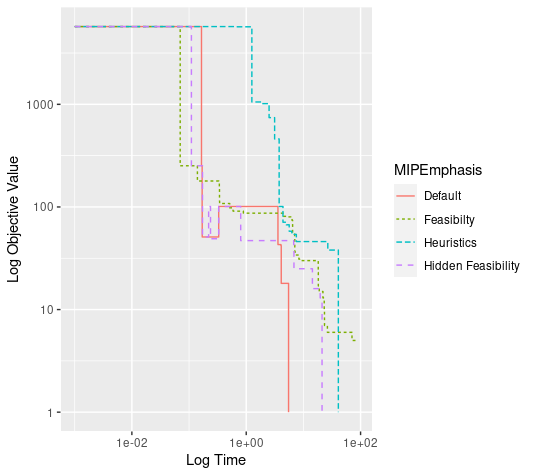
I ran the problem with a 90 second time limit (irrelevant in most cases), using each of the emphasis settings 0, 1, 4 and 5. The following plot (a log-log plot to enhance readability) shows the progress under each setting.

MIPEmphasis 1 ("Feasibility") makes the earliest progress but does not reach the optimal value of 1 within 90 seconds. (At that point, the incumbent value is 5.) Although just shy of one second some of the other levels do a little better than default, overall the default setting reaches the optimal solution fastest and the new setting is worse than the "Hidden Feasibility" setting. We can check the time at which each run (other than with emphasis 1) finds the optimal solution to confirm this.

MIPEmphasis	Time
Default	5.50
Hidden Feasibility	21.19
Heuristics	40.85

 

Test case 2: Typewriter

The second test case is a MIP model for laying out the keyboard of a hypothetical 19th century typewriter. The problem was featured in a series of posts, and the model used here appeared in the last of those posts. As I noted in that post, I was unable to find a provably optimal solution in large part due to a slow moving best bound, so for this demonstration I set a 60 second run limit. The problem seeks to minimize a distance measure. Once again, I'll use a log-log plot to show progress.

All the emphasis settings produce a rapid reduction in the objective function early on. After about a second or so, emphasis 1 (feasibility) seems to do a bit better than the others. Settings 4 and 5 seem to lag a bit. Looking at the final objective values (at the 60 second cutoff), however, it seems that setting 4 (hidden feasibility) did best, and setting 5 (heuristics) slightly outperformed the other settings.

MIPEmphasis	Best
Default	5650882
Feasibilty	5660625
Heuristics	5640159
Hidden Feasibility	5517363

We can also look at node throughput. As a general rule, we would expect that increased use of heuristics would slow down node throughput. One possible exception would be settings that encouraged "diving" (local depth-first search), which might speed up processing of nodes during a dive.

The "heuristics" and "hidden feasibility" settings do in fact process fewer nodes in 60 seconds than does the default setting. The "feasibility" setting process about twice as many nodes as does the default setting, which may mean it does a fair bit of diving.

 

Test case 3: Group Selection

The last example is a group selection problem from yet another earlier post. I tested two slightly different MIP models with five minute time limits. The first variant uses continuous variables for some inherently boolean quantities, while the second variant makes those variables explicitly integer-valued. The second variant seems to be a bit harder to solve, even though they are mathematically equivalent.

The problem is a maximization problem, and none of the runs come remotely near proof of optimality. As noted in the earlier post, nonlinear approaches yielded an objective value of 889.3463, which is apparently optimal.

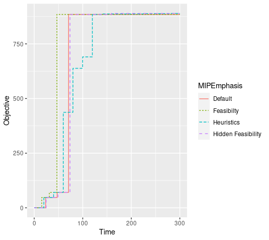
Looking at progress in the incumbent value, we see that all methods make substantial progress at the root node but shortly after the root node appear to bog down. In the first model, there is not much difference among the emphasis settings.

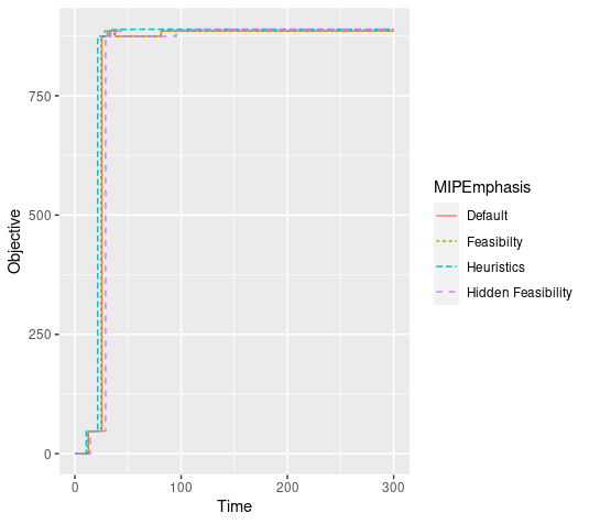
In the second model, the feasibility setting is a bit faster than the other to reach its maximum, and the heuristics setting is slower.

 

In both cases, though, the new "heuristics" setting produces the best objective value after 300 seconds.

MIPEmphasis	Best
Default	885.7781
Feasibilty	885.7781
Heuristics	889.3451
Hidden Feasibility	889.3130

MIPEmphasis	Best
Default	884.6917
Feasibilty	884.6917
Heuristics	889.3392
Hidden Feasibility	889.3130

As for node throughput, the next two plots show that node throughput is clearly greater in the first variant (where inherently boolean variables are treated a continuous with domain [0, 1]), and the "feasibility" setting is again fastest in both variants, while the new "heuristics" setting is slowest.

 

 

Conclusion

Testing on a small set of examples does not tell us much. On the group selection models, where progress is hard to come by after a short time, the new setting produced the best results, but was not much better than the old "hidden feasibility" setting. The same was true on the typewriter problem. So I am still waiting to encounter a problem instance where the new setting will provide a substantial improvement.

Multilogit Fit via LP

 A recent question on OR Stack Exchange has to do with getting an $L_1$ regression fit to some data. (I'm changing notation from the original post very slightly to avoid mixing sub- and super-scripts.) The author starts with $K$ observations $y_1, \dots, y_K$ of the dependent variable and seeks to find $x_{i,k} \ge 0$ ($i=1,\dots,N$, $k=1,\dots,K$) so as to minimize the $L_1$ error $$\sum_{k=1}^K \left|y_k - \sum_{i=1}^N \frac{e^{x_{i,k}}}{\sum_{j=1}^K e^{x_{i,j}}}\right|.$$ The author was looking for a way to linearize the objective function.

The solution I proposed there begins with a change of variables: $$z_{i,k}=\frac{e^{x_{i,k}}}{\sum_{j=1}^K e^{x_{i,j}}}.$$ The $z$ variables are nonnegative and must obey the constraint $$\sum_{k=1}^{K}z_{i, k}=1\quad\forall i=1,\dots,N.$$ With this change of variables, the objective becomes $$\sum_{k=1}^K \left|y_k - \sum_{i=1}^N z_{i,k} \right|.$$ Add nonnegative variables $w_k$ ($k=1,\dots, K$) and the constraints $$-w_k \le y_k - \sum_{i=1}^N z_{i,k} \le w_k \quad \forall k=1,\dots,K,$$ and the objective simplifies to minimizing $\sum_{k=1}^K w_k$, leaving us with an easy linear program to solve.

That leaves us with the problem of getting from the LP solution $z$ back to the original variables $x$. It turns out the transformation from $x$ to $z$ is invariant with respect to the addition of constant offsets. More precisely, for any constants $\lambda_i$ ($i=1,\dots,N$), if we set $$\hat{x}_{i,k}=x_{i,k} + \lambda_i \quad \forall i,k$$ and perform the $x\rightarrow z$ transformation on $\hat{x}$, we get $$\hat{z}_{i,k}=\frac{e^{\lambda_{i}}e^{x_{i,k}}}{\sum_{j=1}^{K}e^{\lambda_{i}}e^{x_{i,j}}}=z_{i,k}\quad\forall i,k.$$ This allows us to convert from $z$ back to $x$ as follows. For each $i$, set $j_0=\textrm{argmin}_j z_{i,j}$ and note that $$\log\left(\frac{z_{i,k}}{z_{i,j_0}}\right) = x_{i,k} - x_{i, j_0}.$$ Given the invariance to constant offsets, we can set $x_{i, j_0} = 0$ and use the log equation to find $x_{i,k}$ for $k \neq j_0$.

Well, almost. I dealt one card off the bottom of the deck. There is nothing stopping the LP solution $z$ from containing zeros, which will automatically be the smallest elements since $z \ge 0$. That means the log equation involves dividing by zero, which has been known to cause black holes to erupt in awkward places. We can fix that with a slight fudge: in the LP model, change $z \ge 0$ to $z \ge \epsilon$ for some small positive $\epsilon$ and hope that the result is not far from optimal.

I tested this with an R notebook. In it, I generated values for $y$ uniformly over $[0, 1]$, fit $x$ using the approach described above, and also fit it using a genetic algorithm for comparison purposes. In my experiment (with dimensions $K=100$, $N=10$), the GA was able to match the LP solution if I gave it enough time. Interestingly, the GA solution was dense (all $x_{i,j} > 0$) while the LP solution was quite sparse (34 of 1,000 values of $x_{i,j}$ were nonzero). As shown in the notebook (which you can download here), the LP solution could be made dense by adding positive amounts $\lambda_i$ as described above, while maintaining the same objective value. I tried to make the GA solution sparse by subtracting $\lambda_i = \min_k x_{i,k}$ from the $i$-th row of $x$. It preserved nonnegativity of $x$ and maintained the same objective value, but reduce density only from 1 to 0.99.

A Greedy Heuristic Wins

 A problem posted on OR Stack Exchange starts as follows: "I need to find two distinct values to allocate, and how to allocate them in a network of stores." There are $n$ stores (where, according to the poster, $n$ can be close to 1,000). The two values (let's call them $x_1$ and $x_2$) must be integer, with $x_1 \in \lbrace 1, \dots, k_1 \rbrace$ and $x_2 \in \lbrace k_1, \dots, k_2 \rbrace$ for given parameters $k_1 < k_2$. Additionally, there is an additional set of parameters $s_{i3}$ and a balance constraint saying $$0.95 g(k_1 e) \le g(x_1, x_2) \le 1.05 g(k_1 e)$$ where $$g(y) = \sum_{i=1} \frac{s_{i3}}{y_i}$$ for any allocation $y$ and $e = (1,\dots, 1).$

The cost function (to be minimized) has the form $$f(x_1, x_2) = a\sum_{i=1}^n \left[ s_{i1}\cdot \left( \frac{s_{i2}}{y_i} \right)^b \right]$$with $a$, $s_{i1}$, $s_{i2}$ and $b$ all parameters and $y_i \in \lbrace x_1, x_2 \rbrace$ is the allocation to store $i$. There are two things to note about $f$. First, the leading coefficient $a (> 0)$ can be ignored when looking for an optimum. Second, given choices $x_1$ and $x_2>x_1$, the cheaper choice at all stores will be $x_1$ if $b < 0$ and $x_2$ if $b > 0$.

It's possible that a nonlinear solver might handle this, but I jumped straight to metaheuristics and, in particular, my go-to choice among metaheuristics -- a genetic algorithm. Originally, genetic algorithms were intended for unconstrained problems, and were tricky to use with constrained problems. (You could bake a penalty for constraint violations into the fitness function, or just reject offspring that violated any constraints, but neither of those approaches was entirely satisfactory.) Then came a breakthrough, the random key genetic algorithm [1]. A random key GA uses a numeric vector $v$ (perhaps integer, perhaps byte, perhaps double precision) as the "chromosome". The user is required to supply a function that translates any such chromosome into a feasible solution to the original problem.

I did some experiments in R, using the GA package to implement a random key genetic algorithm. The package requires all "genes" (think "variables") to be the same type, so I used a double-precision vector of dimension $n_2$ for chromosomes. The last two genes have domains $(1, k_1 + 1)$ and $(k_1, k_2 + 1)$; the rest have domain $(0, 1)$. Decoding a chromosome $v$ proceeds as follows. First, $x_1 = \left\lfloor v_{n+1}\right\rfloor $ and $x_2 = \left\lfloor v_{n+2}\right\rfloor $, where $\left\lfloor z \right\rfloor$ denotes the "floor" (greatest lower integer) of $z$. The remaining values $v_1, \dots, v_{n}$ are sorted into ascending order, and their sort order is applied to the stores. So, for instance, if $v_7$ is the smallest of those genes and $v_{36}$ is the largest, then store $7$ will be first in the sorted list of stores and store $36$ will be last. (The significance of this sorting will come out in a second.)

 

Armed with this, my decoder initially assigns every store the cheaper choice between $x_1$ and $x_2$ and computes the value of $g()$. If $g()$ does not fall within the given limits, the decoder runs through the stores in their sorted order, switching the allocation to the more expensive choice and updating $g()$, until $g()$ meets the balance constraint. As soon as it does, we have the decoded solution. This cheats a little on the supposed guarantee of feasibility in a decoded solution, since there is a (small?) (nearly zero?) chance that the decoding process will fail with $g()$ jumping from below the lower bound to above the upper bound (or vice versa) after some swap. If it does, my code discards the solution. This did not seem to happen in my testing.

 

The GA seemed to work okay, but it occurred to me that I might be over-engineering the solution a bit. (This would not be the first time I did that.) So I also tried a simple greedy heuristic. Since $k_1$ and $k_2$ seem likely to be relatively small in the original poster's problem (whereas $n$ is not), my greedy heuristic loops through all valid combinations of $x_1$ and $x_2$. For each combination, it sets $v_1$ equal to the cheaper choice and $v_2$ equal to the more expensive choice, assigns the cheaper quantity $v_1$ to every store and computes $g()$. It also computes, for each store, the ratio \[ \frac{|\frac{s_{i3}}{v_{2}}-\frac{s_{i3}}{v_{1}}|}{s_{i1}\left(\left(\frac{s_{i2}}{v_{2}}\right)^{b}-\left(\frac{s_{i1}}{v_{1}}\right)^{b}\right)} \]in which the numerator is the absolute change in balance at store $i$ when switching from the cheaper allocation $v_1$ to the more expensive allocation $v_2$, and the denominator is the corresponding change in cost. The heuristic uses these ratios to select stores in descending "bang for the buck" order, switching each store to the more expensive allocation until the balance constraint is met.

Both the GA decoder and the greedy heuristic share the approach of initially allocating every store the cheaper choice and then switching stores to the more expensive choice until balance is attained. My R notebook generates a random problem instance with $n=1,000$ and then solves it twice, first with the GA and then with the greedy heuristic. The greedy heuristic stops when all combinations of $x_1$ and $x_2$ have been tried. Stopping criteria for the GA are more arbitrary. I limited it to at most 1,000 generations (with a population of size 100) or 20 consecutive generations with no improvement, whichever came first.

 

The results on a typical instance were as follows. The GA ran for 49 seconds and got a solution with cost 1065.945. The greedy heuristic needed only 0.176 seconds to get a solution with cost 1051.735. This pattern (greedy heuristic getting a better solution in much less time) repeated across a range of random number seeds and input parameters, including switching between positive and negative values of $b$.

If you are interested, you can browse my R notebook (which includes both code and results).

 

[1] Bean, J. C. (1994). Genetic Algorithms and Random Keys for Sequencing and Optimization. ORSA Journal on Computing, 6, 154-160.

Installing Rcplex and cplexAPI

I've previously mentioned solving MIP models in R, using CPLEX. In one post [1], I used the OMPR package, which provides a domain specific language for model construction. OMPR uses the ROI package, and in particular the ROI.plugin.cplex package, to communicate with CPLEX. That, in turn, uses the Rcplex package. In another post [2], I used Rcplex directly. Meanwhile, there is still another package, cplexAPI, that provides a low-level API to CPLEX.

Both Rcplex and cplexAPI will install against CPLEX Studio 12.8 and earlier, but neither one installs with CPLEX Studio 12.9 or 12.10. Fortunately, IBM's Daniel Junglas was able to hack solutions for both of them. I'll spell out the steps I used to get Rcplex working with CPLEX 12.10. You can find the solutions for both in the responses to this question on the IBM Decision Optimization community site. Version information for what follows is: Linux Mint 19.3; CPLEX Studio 12.10; R 3.6.3; and Rcplex 0.3-3. Hopefully essentially the same hack works with Windows.

1. Download Rcplex_0.3-3.tar.gz, put it someplace harmless (the Downloads folder in my case, but /tmp would be fine) and expand it, producing a folder named Rcplex.
2. Go to the Rcplex folder and open the 'configure' file in a text editor (one you would use for plain text files).
3. Line 1548 should read as follows:
   

   CPLEX_LIBS="-L${CPLEXLIBDIR} `${AWK} 'BEGIN {FS = " = "} /^CLNFLAGS/ {print $2}' ${CPLEX_MAKEFILE}`"

   .
   Replace it with
   

   CPLEX_LIBS="-L${CPLEXLIBDIR} `${AWK} 'BEGIN {FS = " = "} /^CLNFLAGS/ {print $2}' ${CPLEX_MAKEFILE} | sed -e 's,\$(CPLEXLIB),cplex,'`"

   .
   Save the modified file.
   
4. Open a terminal in the parent directory of the Rcplex folder and run the following command:
   

   R CMD INSTALL --configure-args="--with-cplex-dir=.../CPLEX_Studio1210/cplex/" ./Rcplex

   .
   Adjust the file path (particularly the ...) so that it points to the 'cplex' directory in your CPLEX Studio installation (the one that has subdirectories named "bin", "examples", "include" etc.).
5. Assuming there were no error messages during installation, you should be good to go.
   

[1] https://orinanobworld.blogspot.com/2016/11/mip-models-in-r-with-ompr.html

[2] https://orinanobworld.blogspot.com/2020/08/a-group-selection-problem.html

Update: Version 1.4.0 of cplexAPI, released on 2020-09-21, installs correctly against CPLEX 12.10 (and presumably 12.9), at least on my system (Linux Mint).

A Group Selection Problem

Someone posted an interesting question about nonlinear integer programming with grouped binary variables on Stack Overflow, and it drew multiple responses. The problem is simple to state. You have 52 binary variables $x_i$ partitioned into 13 groups of four each, with a requirement that exactly one variable in each group take the value 1. So the constraints are quite simple:

\begin{align*} x_{1}+\dots+x_{4} & =1\\ x_{5}+\dots+x_{8} & =1\\ \vdots\\ x_{49}+\dots+x_{52} & =1. \end{align*}

The objective function is a cubic function of the form

\[ \left(\alpha\sum_{i}a_{i}x_{i}\right)\times\left(\beta\sum_{j}b_{j}x_{j}+\beta_{0}\right)\times\left(\gamma\sum_{k}c_{k}x_{k}+\gamma_{0}\right) \] where $\alpha = 1166/2000$, $\beta = 1/2100$, $\beta_0 = 0.05$, $\gamma = 1/1500$ and $\gamma_0 = 1.5$. (In the original post, there is a minus sign in front of the function and the author minimizes; for various reasons I am omitting the minus sign and maximizing here.) Not only is the objective nonlinear, it is nonconvex if minimizing (nonconcave if maximizing). The author of the question was working in R.

Fellow blogger Erwin Kalvelagen solved the problem with a variety of nonlinear optimizers, obtaining a solution with objective value -889.346. Alex Fleischer of IBM posted an answer with the same objective value, using a constraint programming model written in OPL and solved with CP Optimizer.

My initial thought was to linearize the objective function by introducing continuous variables $y_{ij} = x_i \cdot x_j$ and $z_{ijk} = x_i \cdot x_j \cdot x_k$ with domain [0,1]. Many of those variables can be eliminated, due in part to symmetry ($y_{ij} = y_{ji}$, $z_{ijk} = z_{ikj}=\dots=z_{kji}$ and in part due to the observation that $y_{ii}=z_{iii}=x_i$. Also useful is that for $i<j<k$ $z_{ijk}=x_i \cdot y_{jk}$. I have an R notebook that you can download, in which I build the model using standard linearizations for the product of two binarys, then try to solve it with CPLEX using the Rcplex package (and the Matrix package, which allows a sparse representation of the constraint matrix). The results were, shall we say, unspectacular. With a five minute time limit (much longer than what Erwin or Alex needed), CPLEX found an incumbent with value 886.8748 (not bad but not optimal) and a rather dismal optimality gap of 146.5% (due mainly to a loose and slow moving bound).

Out of curiosity, I took a second shot using a genetic algorithm and the GA package for R. I was geeked to see that the GA package includes both an island model (using parallel processing) and a permutation variant (which lets me use permutations of the indices 1 to 52 as chromosomes with no extra work on my part). The permutation approach allows me to treat a chromosome as a prioritization of the 52 binary variables, which I decode into a solution $x$ by scanning the $x_i$ in priority order and setting each to 1 if and only none of the other variables in its group of four has been set to 1. That R notebook is also available for download.

As a metaheuristic, the GA does not offer a proof of optimality, and in fact may or may not find the optimal solution. With my inspired choice of random number seed (123), I matched Erwin's and Alex's solution (889.3463). The settings I used resulted in a run time of about 36 seconds on my PC, more than half of which was spent after the best solution had been found. It's still slower than what Erwin and Alex achieved, but it is a "pure R" solution, meaning it requires nothing besides open-source R packages.

Multiobjective Optimization in CPLEX

In my previous post, I discussed multiobjective optimization and ended with a simple example. I'll use this post to discuss some of the new (as of version 12.9) features in CPLEX related to multiobjective optimization, and then apply them to the example from the previous post. My Java code can be downloaded from my GitLab repository.

Currently (meaning as of CPLEX version 12.10), CPLEX supports multiple objectives in linear and integer programs. It allows mixtures of "blended" objective functions (weighted combinations of original criteria) and "lexicographic" hierarchical objectives. Basically, you set one or more hierarchy (priority) levels, and in each one you can have a single criterion or a weighted combination of criteria. So the "classical" preemptive priority approach would involve multiple priority levels with a single criterion in each, while the "classical" weighted combination approach would involve one priority level with a blended objective in it. Overall, you are either maximizing or minimizing, but you can use negative weights for criteria that should go the opposite direction of the rest. In the example here, which is a minimization problem, the third priority level gives maximum provider utilization a weight of +1 (because we want to minimize it) and minimum provider utilization a weight of -1 (because we want to maximize it).

There are some limitations to the use of multiple objectives. The ones I think are of most general interest are the following:

• objectives and constraints must be linear (no quadratic terms); and
• all generic callbacks and legacy information callbacks can be used, but other legacy callbacks, and in particular legacy control callbacks (branch callbacks, cut callbacks etc.) cannot be used. So if you need to use callbacks with a multiobjective problem, now would be a good time to learn the new generic callback system.

Every criterion you specify has a priority level and, within that priority level, a weight. A feature that I appreciate, and which I will use in the code, is that you can also specify an absolute and/or a relative tolerance for each criterion. The tolerances tell CPLEX how much it can sacrifice in that criterion to improve lower priority criteria. The default tolerance is zero, meaning higher priority criteria must be optimized before lower priority criteria are even considered. A nonzero tolerance basically tells CPLEX that is allowed to sacrifice some amount (either an absolute amount or a percentage of the optimal value) in that criterion in order to improve lower priority criteria.

Defining the variables and building the constraints of a multiobjective model is no different from a typical single criterion model. Getting the solution after solving the model is also unchanged. The differences come mainly in how you specify the objectives and how you invoke the solver.

To build the objective function, you need to use one of the several overloads of IloCplex.staticLex(). They all take as first argument a one dimensional array of expressions IloNumExpr[], and they all return an instance of the new interface IloCplexMultiCriterionExpr. In addition to an array of objective expressions, one of the overloads lets you also specify arrays of weights, priorities and tolerances (absolute and relative). That's the version used in my sample code. 

This brings me to a minor inconvenience relative to a conventional single objective problem. Ordinarily, I would use IloCplexModeler.addMinimize(expr) or IloCplexModeler.addMaximize(expr) to add an objective to a model, where expr is an instance of IloNumExpr. I naively thought to do the same here, using the output of staticLex() as the expression, but that is not (currently) supported. There's no overload of addMinimize() or addMaximize() that accepts a multicriterion expression. So it's a three step process: use cplex.staticLex(...) to create the objective and save it to a temporary variable (where cplex is your IloCplex instance); pass that variable to either cplex.minimize(...) or cplex.maximize(...) and save the resulting instance of IloObjective in a temporary variable; and then invoke cplex.add(...) on that variable.

When you are ready to solve the model, you invoke the solve() method on it. You can continue to use the version of solve() that takes no arguments (which is what my code does), or you can use a new version that takes as argument an array of type IloCplex.ParameterSet[]. This allows you to specify different parameter settings for different priority levels.

Other methods you might be interested in are IloCplex.getMultiObjNSolves() (which gets the number of subproblems solved) and IloCplex.getMultiObjInfo() (which lets you look up a variety of things that I really have not explored yet).

The output from my code (log file), which is in the repository, is too lengthy to show here, but if you want you can use this link to open it in a new tab. Here's a synopsis. I first optimized each of the three objective functions separately. (Recall that maximum and minimum provider utilization are blended into one objective.) This gives what is sometimes referred to as the "Utopia point" or "ideal point". This is column "U" in the table below. Next, I solved the prioritized multiobjective problem. The results are in column "O" of the table. Finally, to demonstrate the ability to be flexible with priorities, I resolved the multiobjective problem using a relative tolerance of 0.1 (10%) for the top priority objective (average distance traveled) and 0.05 (5%) for the second priority objective (maximum distance traveled). Those results are in column "F".

	U	O	F
Avg. distance	14.489	14.489	15.888
Max distance	58.605	58.605	60.000
Utilization spread	0.030	0.267	0.030
Max utilization	0.710	0.880	0.710
Min utilization	0.680	0.613	0.680

There are a few things to note.

1. The solution to the multiobjective model ("O") achieved the ideal values for the first two objectives. One would expect to match the ideal value on the highest priority objective; matching on the second objective was luck. The third objective (utilization spread) was, not surprisingly, somewhat worse than the ideal value.
2. Absolute and relative tolerances appear to work the same way that absolute and relative gap tolerances do: if a solution is within either absolute or relative tolerance of the best possible value on a higher priority objective, it can be accepted. In the third run, I set relative tolerances but let the absolute tolerances stay at default values.
3. The relative tolerances I set in the last run would normally allow CPLEX to accept a solution with an average travel distance as large as $(1 + 0.1)*14.489 = 15.938$ and a maximum travel distance as large as $(1 + 0.05)*58.605 = 61.535$. There is a constraint limiting travel distance to at most 60, though, which supersedes the tolerance setting.
4. The "flexible" solution (column "F") exceeds the ideal average distance by about 9.7%, hits the cap of 60 on maximum travel distance, and actually achieves the ideal utilization spread. However, without knowing the ideal point you would not realize that last part. I put a fairly short time limit (30 seconds) on the run, and it ended with about a 21% gap due to a very slow-moving best bound.

I'll close with one last observation. At the bottom of the log, after solving the "flexible" variant, you will see the following lines.

Solver status = Unknown.
Objective 0: Status = 101, value = 14.489, bound = 14.489.
Objective 1: Status = 101, value = 58.605, bound = 58.605.
Objective 2: Status = 107, value = 0.030, bound = 0.023.
Final value of average distance traveled = 15.888.
Final value of longest distance traveled = 60.000.
Final value of maximum provider utilization = 0.710.
Final value of minimum provider utilization = 0.680.

The first four lines are printed by CPLEX, the last four by my code. Note the mismatch in objective values of the first two criteria (bold for CPLEX, italic for my results). CPLEX prints the best value it achieved for each objective before moving on to lower priority objectives. When you are using the default tolerances of zero (meaning priorities are absolute), the printed values will match what you get in the final solution. When you specify non-zero tolerances, though, CPLEX may "give back" some of the quality of the higher priority results to improve lower priority results, so you will need to recover the objective values yourself.

Multiobjective Optimization

Multiobjective optimization (making "optimal" decisions involving multiple, frequently conflicting, criteria) is a big subject. I will only nibble at the fringes of it here. In the next post, I'll describe recent additions to CPLEX that facilitate solving some multiobjective problems.

Among the various approaches to multiobjective problems, two are probably the most common, weighting and prioritization. The first approach is to merge the various criteria into a single one, usually (almost always?) by taking a weighted sum of the criteria. The CPLEX documentation refers to this as a blended objective. For this to make sense, the units of the various criteria really should be commensurable (e.g., all monetary values), but I'm pretty sure having criteria that are not commensurable doesn't stop people from trying. The weights serve two roles. First, they bring the units into some semblance of parity (so if $f()$ is in dollars and $g()$ in millions of dollars, $g()$ gets a weight roughly on millionth the size of the weight of $f()$). Second, they convey relative importance of various criteria.

The second approach is to prioritize the criteria. The solver initially optimizes the highest priority criterion, without regard to any others. Once an optimal value of the highest priority criterion is known, maintaining that value becomes a constraint, and the solver moves to the second highest priority criterion, and so on. The CPLEX documentation refers to this as a lexicographic objective, meaning that the objective function is vector-valued rather than scalar-valued, and optimization means achieving the lexicographically largest or smallest objective vector possible. A variant of this allows a little "slippage" in the value of each criterion, so that for example the solver can accept a solution that is 1% below optimal on the first criterion in return for optimizing the second criterion. A key limitation here is the solver will trade any amount of degradation in a lower priority criterion, no matter how much, for any improvement in a higher priority criterion, no matter how small.

Although they are not relevant to the recent CPLEX additions, I will mention two other approaches. One is a variant of the priority method, known as goal programming (GP). This was originally developed as an extension of linear programming, but the same general approach can be extended to problems with integer variables. The user sets target levels for each criterion, and then prioritizes them. If a goal is underachieved, work on meeting lower priority goals cannot sacrifice any amount of the higher priority criterion. On the other hand, if a goal is overachieved, any portion of the overachievement can be sacrificed in the quest to reach a lower priority goal. An interesting attribute of goal programming is that the same criterion can be used with more than one goal. Suppose that you are building a GP model allocating a budget to various conservation projects. Your highest priority goal might be to allocate at least 50% of the budget to projects in underserved communities (USCs, to save me typing, with apologies to the universities of South Carolina and Southern Califonia). Your second highest priority goal might be to allocate at least 30% of the budget to projects with matching funds from outside sources. Your third highest priority goal might be to allocate at least 75% of the budget to USCs. The other approach is to investigate the Pareto frontier, the set of all solutions for which no other solution does as well in all criteria and better in at least one. In essence, you want to present the decision-maker with the entire Pareto frontier and say "here, pick one". In practice, computing the Pareto frontier can be very computationally expensive, and trying to make sense of it might cause the decision maker to melt down.

To close this post, I'll pose a small sample problem and formulate the model for it. Suppose that we have $N$ patients in a health care system and $M$ providers, and that each patient needs to be assigned to a single provider. Provider $j$ has a limit $c_j$ on the number of patients they can handle. (To keep the example simple, and at the expense of some realism, we treat all patients as identical with regard to their capacity consumption.) We are given a matrix $D\in \mathbb{R}^{N\times M}$ of distances from patients to providers, as well as a cap $D_{max}$ on the distance that a patient can be required to travel. There are four criteria to be considered:

• the average distance patients will travel (minimize, highest priority);
• the maximum distance any patient must travel (minimize, second highest priority);
• the maximum utilization of any provider as a fraction of their capacity (minimize, tied for third highest priority); and
• the minimum utilization of any provider as a fraction of their capacity (maximize, tied for third highest priority).

So we have a mix of three things to minimize and one to maximize, with the last two criteria combining to somewhat level the workload across providers. 

Let $x_{ij}$ be 1 if patient $i$ is assigned to provider $j$ and 0 if not, let $w$ be the longest distance traveled by any patient, let $y_j$ be the fraction of provider $j$'s capacity that is utilized, and let $z_{lo}$ and $z_{hi}$ be the minimum and maximum capacity utilization rates, respectively (where 0 means the provider is unused and 1 means the provider is operating at capacity). The objective expression is $f\in\mathbb{R}^3$, whose lexicographic minimum we seek, where

\[ f=\left[\begin{array}{c} \frac{1}{N}\sum_{i=1}^{N}\sum_{j=1}^{M}d_{ij}x_{ij}\\ w\\ z_{hi}-z_{lo} \end{array}\right]. \]

The first and second components of $f$ are the average and maximum client travel distances. The third component is a weighted mix of maximum and minimum provider utilization, where the weights (+1, -1) are equal in magnitude to reflect the equal importance I am assigning to them and the negative coefficient for minimum utilization allows it to be maximized in what is otherwise a minimization problem.

The constraints of the model are easy to state:

\begin{align*} \sum_{j=1}^{M}x_{ij} & =1\quad\forall i\in\left\{ 1,\dots,N\right\} & (1)\\ d_{ij}x_{ij} & \le w\quad\forall i\in\left\{ 1,\dots,N\right\} ,\forall j\in\left\{ 1,\dots,M\right\} & (2)\\ \frac{1}{c_{j}}\sum_{i=1}^{N}x_{ij} & =y_{j}\quad\forall j\in\left\{ 1,\dots,M\right\} & (3)\\ y_{j} & \le z_{hi}\quad\forall j\in\left\{ 1,\dots,M\right\} & (4)\\ y_{j} & \ge z_{lo}\quad\forall j\in\left\{ 1,\dots,M\right\} & (5)\\ x & \in\left\{ 0,1\right\} ^{N\times M} & (6)\\ x_{ij} & =0\quad\forall i,j\ni d_{ij}>D_{max} & (7)\\ y & \in\left[0,1\right]^{M} & (8)\\ z_{hi},z_{lo} & \in\left[0,1\right] & (9)\\ w & \in\left[0,D_{max}\right] & (10) \end{align*} 

• Constraint (1) ensures that each patient is assigned to exactly one provider.
• Constraint (2) defines $w$, the maximum distance traveled.
• Constraint (3) defines the fraction $y_j$ of capacity used at each provider $j$.
• Constraints (4) and (5) define $z_{lo}$ and $z_{hi}$.
• Constraints (6), (8), (9) and (10) define variable domains. The upper bound of 1 for $y_j$ in (8) ensures that no provider is assigned more patients than their capacity allows.
• Constraint (7) enforces the travel distance limit $D_{max}$ by preventing any assignments that would violate the limit (effectively removing those assignment variables from the model).

In the next post, I will show how to solve the model using CPLEX (with, as usual, the Java API).

 

A Partitioning Problem

 A recent question on Mathematics Stack Exchange dealt with reducing the number of sets in a partition of a set of items. I'll repeat it here but with slightly different terminology from the original question. You start with $N$ items partitioned into $M$ disjoint sets. Your goal is to generate a smaller partition of $K < M$ sets (which I will henceforth call "collections" to distinguish them from the original sets). It is required that all items from any original set end up in the same collection (i.e., you cannot split the original sets). The criterion for success is that "the new [collection] sizes should be as close to even as possible".

This is easily done with an integer programming model. The author of the question thought about minimizing the variance in the collection sizes, which would work, but I'm fond of keeping things linear, so I will minimize the range of collection sizes. I'll denote the cardinality of original set $i$ by $n_i$. Let $x_{ij}$ be a binary variable which is 1 if set $i\in \lbrace 1,\dots, M\rbrace$ is assigned to collection $j\in \lbrace 1,\dots,K\rbrace$  and 0 if not. Let $y$ and $z$ denote the sizes of the smallest and largest collections. Finally, for $j\in \lbrace 1,\dots,K\rbrace$ let $s_j$ be the size (cardinality) of collection $j$. A MILP model for the problem is the following:

\begin{align} \min\,z-y\\ \textrm{s.t. }\sum_{j=1}^{K}x_{ij} & =1\;\; \forall i\in\left\{ 1,\dots M\right\} \\ \sum_{i=1}^{M}n_{i}x_{ij} & =s_{j}\;\; \forall j\in\left\{ 1,\dots,K\right\} \\ s_{j} & \le z\;\; \forall j\in\left\{ 1,\dots,K\right\} \\ s_{j} & \ge y\;\; \forall j\in\left\{ 1,\dots,K\right\} \\ y,z,s_{\cdot} & \ge0\\ x_{\cdot\cdot} & \in\left\{ 0,1\right\} \end{align} 

The author of the question also indicated an interest in "fast greedy approximate solutions" (and did not specify problem dimensions). The first greedy heuristic that came to my mind was a simple one. Start with $K$ empty collections and sort the original sets into descending size order. Now assign each set, in turn, to the collection that currently has the smallest size (breaking times whimsically). Why work from largest to smallest set? There will be times when you will want to offset a large set in one collection with two or more smaller sets in another collection, and that will be easier to do if you start big and keep the smaller sets in reserve as long as is possible. Rob Pratt, owner of a rather massive reputation score on MSE, correctly noted that this is equivalent to the "longest processing time" heuristic for assigning jobs to machines so as to minimize makespan.

I put together an R notebook to test this "greedy" heuristic against the optimization model (solved with CPLEX). The notebook uses Dirk Schumacher's OMPR package for building the MILP model. It in turn uses the ROI package (which requires the Rcplex package) in order to communicate with CPLEX. On a test run using nice, round values of $N$, $M$ and $K$ that all ended in zeros (and in particular where $K$ divided evenly into both $M$ and $N$), the greedy heuristic nearly found the optimal solution. When I switched to less round numbers ($N=5723$, $M=137$, $K=10$), though, the heuristic did not fare as well. It was fast (well under one second on my PC) but it produced a solution where collection sizes ranged from 552 to 582 (a spread of 30), while CPLEX (in about 21 seconds) found an optimal solution where all collections had size either 572 or 573 (spread of 1). So I tacked on a second heuristic to refine the solution of the first heuristic. The second heuristic attempts pairwise swaps of the smallest set from the smallest collection with a larger set from a larger collection (trying collections in descending size order). Swaps are constrained not to leave the second collection (the one donating the larger set) smaller than the first collection started out. The intuition is to shrink the range by making the smallest collection bigger while shrinking the largest collection if possible and, if not, at least some collection that is larger than the smallest one. The new heuristic also ran in well under one second and shrank the range of collection sizes from 30 to 3 -- still not optimal, but likely good enough for the application the original questioner had in mind.

You are free to use the R code (which can be extracted from the notebook linked above) under the Creative Commons license that governs the blog.

Firefox and the New Blogger Interface

Blogger has a (relatively) new interface, to which I switched a while back. The one major annoyance I found was that clicking the "Preview" button while editing a post did not actually generate a preview. I got a notification (lower left) that the preview was being prepared, and then ... nothing. To get a preview, I had to save my work, exit the edit screen (going back to the Blogger control panel), and do the preview there.

It wasn't just me, either. Checking the Blogger help community, I found a ton of posts about this, on pretty much all operating systems and browsers, with some dated this month. A tip about fixing the problem on Safari worked for me. The key (somewhat obvious in hindsight) is that Blogger needs permission to open a pop-up. This was not entirely obvious to me, since I don't consider opening a tab the same as opening a pop-up, but so be it. In Firefox, with any Blogger screen displayed, click the padlock icon in the URL bar, and under "Permissions" allow the site to open pop-ups.

Other users said they had the same problem with Chrome, which is interesting in that preview works fine for me on Chrome, and I don't recall giving explicit permission there. At any rate, I seem to be back in business.

And yes, I previewed this entry before posting it.

Longest Increasing Subsequence

In a recent blog post (whose title I have shamelessly appropriated), Erwin Kalvelagen discusses a mixed-integer nonlinear programming formulation (along with possible linearizations) for a simple problem from a coding challenge: "Given an unsorted array of integers, find the length of longest increasing subsequence." The challenge stipulates at worst $O(n^2)$ complexity, where $n$ is the length of the original sequence. Erwin suggests the intent of the original question was to use dynamic programming, which makes sense and meets the complexity requirement.

I've been meaning for a while to start fiddling around with binary decision diagrams (BDDs), and this seemed like a good test problem. Decision diagrams originated in computer science, where the application was evaluation of possibly complicated logical expressions, but recently they have made their way into the discrete optimization arena. If you are looking to familiarize yourself with decision diagrams, I can recommend a book by Bergman et al. [1].

Solving this problem with a binary decision diagram is equivalent to solving it with dynamic programming. Let $[x_1, \dots, x_n]$ be the original sequence. Consistent with Erwin, I'll assume that the $x_i$ are nonnegative and that the subsequence extracted must be strictly increasing.

We create a layered digraph in which each node represents the value of the largest (and hence most recent) element in a partial subsequence, and has at most two children. Within a layer, no two nodes have the same state, but nodes in different layers can have the same state. We have $n+2$ layers, where in layer $j\in\lbrace 1,\dots,n \rbrace$ you are deciding whether or not to include $x_j$ in your subsequence. One child, if it exists, represents the state after adding $x_j$ to the subsequence. This child exists only if $x_j$ is greater than the state of the parent node (because the subsequence must be strictly increasing). The other child, which always exists, represents the state when $x_j$ is omitted (which will be the same as the state of the parent node). Layer 1 contains a root node (with state 0), layer $n+1$ contains nodes corresponding to completed subsequences, and layer $n+2$ contains a terminal node (whose state will be the largest element of the chosen subsequence). Actually, you could skip layer $n+1$ and follow layer $n$ with the terminal layer; in my code, I included the extra layer mainly for demonstration purposes (and debugging).

In the previous paragraph, I dealt a card off the bottom of the deck. The state of a node in layer $j$ is the largest element of a partial subsequence based on including or excluding $x_1,\dots,x_{j-1}$. The sneaky part is that more than one subsequence may be represented at that node (since more than one subsequence of $[x_1,\dots,x_{j-1}]$ my contain the same largest element). In addition to the state of a node, we also keep track at each node of the longest path from the root node to that node and the predecessor node along the longest path, where length is defined as the number of yes decisions from the root to that node. So although multiple subsequences may lead to the same node, we only care about one (the longest path, breaking ties arbitrarily). Note that by keeping track of the longest path from root to each node as we build the diagram, we actually solve the underlying problem during the construction of the BDD.

The diagram for the original example ($n=8$) is too big to fit here, so I'll illustrate this using a smaller initial vector: $x=[9, 2, 5, 3]$. The BDD is shown below (as a PDF file, so that you can zoom in or out while maintaining legibility).

The first four layers correspond to decisions on whether to use a sequence entry or not. (The corresponding entries are shown in the right margin.) Nodes "r" and "t" are root and terminus, respectively. The remaining nodes are numbered from 1 to 14. Solid arrows represent decisions to use a value, so for instance the solid arrow from node 4 to node 8 means that 5 ($x_3$) has been added to the subsequence. Dashed arrows represent decisions not to use a value, so the dashed arrow from node 4 to node 7 means that 5 ($x_3$) is not being added to the subsequence. Dotted arrows (from the fifth layer to the sixth) do not represent decisions, they just connect the "leaf" nodes to the terminus.

The green(ish) number to the lower left of a node is the state of the node, which is the largest element included so far in the subsequence. The subsequence at node 4 is just $[2]$ and the state is 2. At node 7, since we skipped the next element, the subsequence and state remain the same. At node 8, the subsequence is now $[2, 5]$ and the state changes to 5.

The red numbers $d_i:p_i$ to the lower right of a node $i$ are the distance (number of solid arcs) from the root to node $i$ along the longest path ($d_i$) and the predecessor of node $i$ on the longest path ($p_i$). Two paths converge at $i=13$: a path $r \dashrightarrow 2 \rightarrow 4 \dashrightarrow 7 \rightarrow 13$ of length 2 and a path $r \dashrightarrow 2 \dashrightarrow 5 \dashrightarrow 9 \rightarrow 13$ of length 1. So the longest path to node 13 has length 2 and predecessor node 7. Backtracking from the terminus (distance 2, predecessor either 12 or 13), we get optimal paths $r \dashrightarrow 2 \rightarrow 4 \rightarrow 8 \dashrightarrow 12 \dashrightarrow t$ (subsequence $[2, 5]$) and $r \dashrightarrow 2 \rightarrow 4 \dashrightarrow 7 \rightarrow 13 \dashrightarrow t$ (subsequence $[2, 3]$), the latter shown in blue.

In addition to the original example from the coding challenge ($n=8$), Erwin included an example with $n=100$ and longest increasing subsequence length 15. (There are multiple optimal solutions to both the original example and the larger one.) Gurobi solved the larger example to proven optimality in one second (probably less, since the output likely rounded up the time). My highly non-optimized Java code solved the $n=100$ example in 6 ms. on my PC (not including the time to print the results).

BDDs can get large in practice, with layers growing combinatorially. In this case, however, that is not a problem. Since the state of a node is the largest value of a subsequence, there can be at most $n$ different states. Given the stipulation that no two nodes in a layer have the same state, that means at most $n$ states in a layer. For Erwin's example with $n=100$, the largest layer in fact contained 66 nodes.

As I said earlier, using the BDD here is equivalent to using dynamic programming. With $n+2$ layers, at most $n$ nodes in a layer, and two operations on each node (figuring out the state and path length of the "yes" child and the "no" child), the solution process is clearly $O(n^2)$.

[1] D. Bergman, A. A. Cire, W.-J. van Hoeve and J. Hooker. Decision Diagrams for Optimization (B. O’Sullivan and M. Wooldridge, eds.).  Springer International Publishing AG, 2016.

Mint 20 Upgrade Hiccup

Okay, "hiccup" might be an understatement. Something beginning with "cluster" might be more appropriate.

I tried to upgrade my MythTV backend box from Linux Mint 19.3 to Mint 20, using the Mint upgrade tool. Even on a fairly fast machine with a fast Internet connection and not much installed on it (MythTV plus the applications that come with Mint), this takes hours. A seemingly endless series of commands scroll in a terminal, and I don't dare walk away for too long, less the process stop waiting for some input from me (it periodically needs my password) or due to a glitch.

Speaking of glitches, I noticed that the scrolling stopped and the process seemed to freeze just after a couple of lines about installing symlinks for MySQL and MariaDB, two database programs. MariaDB, which I've never had installed before, is apparently a fork of MySQL. MythTV uses MySQL as its database manager. Before upgrading, I had killed the MythTV back end, but I noticed that the MySQL server was still running. On a hunch, I opened a separate terminal and shut down the MySQL server. Sure enough, the upgrade process resumed, with a message about a cancelled job or something, which I think referred to MariaDB. Whether this contributed to the unfolding disaster I do not know.

After a reboot, the good news was that everything that should start did start, and the frontend was able to see and play the recorded TV shows. The bad news was that (a) the backend got very busy doing a lot of (alleged) transcoding and scanning for commercials that should not have been necessary (having already been done on all recorded shows) and (b) I could not shut down, because the backend thought it was in a "shutdown/wakeup period", meaning (I think) that it thought it needed to start recording soon -- even though the next scheduled recording was not for a couple of days, and the front end was showing the correct date and time for the next recording. So I think the switch from MySQL to MariaDB somehow screwed up something in the database.

From there, things got worse. I had backed up the database, so I tried to restore the backup (using a MythTV script for just that purpose). The script failed because the database already contained data. Following suggestions online, I dropped the relevant table from the database and tried to run an SQL script (mc.sql) to restore a blank version of the table. No joy -- I needed the root MySQL password, and no password I tried would work. There is allegedly a way to reset the root password in a MySQL database, but that didn't work either, and in fact trying to shut the server down using "sudo service mysql stop" did not work (!). The only way to get rid of the service was to use "sudo pkill mysqld".

Fortunately, timeshift was able to restore the system to its pre-upgrade state (with a little help from a backup of the MythTV database and recordings folder). For reasons I do not understand (which describes pretty much everything discussed here), restoring the database backup did not cause MythTV to remember this week's schedule of recordings, but as soon as I reentered one (using MythWeb) it remembered the rest. And I thought my memory was acting a bit quirky ...

Zoom on Linux

Thanks to the pandemic, I'm been spending a lot of time on Zoom lately, and I'm grateful to have it. The Zoom Linux client seems to be almost as good as the other clients. The only thing that I know is missing is virtual backgrounds, which I do not particularly miss.

That said, I did run into one minor bug (I think). It has to do with what I think is called the "panel". (I've found it strangely hard to confirm this, despite a good bit of searching.) What I'm referring to is a widget that sits off to one side (and can be moved by me) when Zoom is running full screen and a presenter is holding the "spotlight" (owning the bulk of the window). The panel has four buttons at the top that let me choose its configuration. Three of them will show just my video (small, medium or large). The fourth one will show a stack of four videos, each a participant (excluding the presenter), with mine first and the other three selected by some rule I cannot fathom. (Empirical evidence suggests it is not selecting the three best looking participants.) Showing my camera image isn't exactly critical, but it's somewhat reassuring (meaning I know my camera is still working, and I'm in its field of view).

I'm running Zoom on both a desktop and a laptop, the latter exclusively for online taekwondo classes. On my desktop, the panel behaves as one would expect. On my laptop, however, the panel window assigned to my camera was intermittently blanking out. Randomly moving the cursor around would bring the image back (temporarily). This happened regardless of what panel configuration or size I chose.

On a hunch, I disabled the screen lock option on the laptop (which would normally blank the screen or show a lock screen if the laptop sat idle for too long. To be the clear, even with no keyboard/mouse input from me, the laptop was not showing the lock screen or sleeping -- the main presenter was never interrupted. It was just my camera feed that seemed to be napping. That said, disabling the lock screen seems to have helped somewhat. If the panel is showing only my camera, it still blanks after some amount of "idle" time; but if the panel is set to show a stack of four cameras (including mine), mine does not seem to blank out any more.

It's still a mystery to me why mine blanks when it's the only one in the panel, although it's clear there's a connection to my not providing any keyboard or mouse input for a while. The blanking never happens on my desktop. They're both running Linux Mint (the laptop having a somewhat newer version), and they're both running the latest version of the Zoom client. The laptop has a built-in camera whereas the desktop has a USB webcam. The desktop, unsurprisingly, has a faster processor, and probably better graphics. My typical desktop Zoom usage does not involve extended periods of inactivity on my part (if I'm not doing something useful as part of the call, I'm surreptitiously checking email or playing Minesweeper), so the lack of blanking on the laptop may just be lack of opportunity. It might be a matter of the desktop having better hardware. It might just be some minor computer deity figuring it's more entertaining to annoy me during a workout than during a meeting. Anyway, turning off the screensaver got rid of at least part of the problem. If anyone knows the real reason and/or the right fix, please leave a comment.

An Idea for an Agent-Based Simulation

I don't do agent-based simulations (or any other kind of simulations these days), so this is a suggested research topic for someone who does.

A number of supermarkets and other large stores have instituted one-way lanes, presumably thinking this will improve physical distancing of customers. I just returned from my local Kroger supermarket, where the narrower aisles have been marked one-way, alternating directions, for a few weeks now. The wider aisles remain bidirectional (or multidirectional, the way some people roll). Despite having been fairly clearly marked for weeks, I would say that close to half of all shoppers (possibly more than half) are either unaware of the direction limits or disregard them. Kroger offers a service where you order online, their employees grab and pack the food (using rather large, multilevel rolling carts), and then bring it out to your waiting car. Kroger refers to this as "Pickup" (formerly "Clicklist"). Interestingly, somewhere between 70% and 90% of the employees doing "Pickup" shopping that I encountered today were going the wrong direction on the directional aisles.

My perhaps naive thought is that unidirectional aisles are somewhere between useless and counterproductive, even if people obey the rules. That's based on two observations:

1. the number of people per hour needing stuff from aisle 13 is unaffected by any directional restrictions on the aisle; and
2. obeying the rules means running up extra miles on the cart, as the shopper zips down aisle 12 (which contains nothing he wants) in order to get to the other end, so that he can cruise aisle 13 in the designated direction.

Of course, OR types could mitigate item 2 by solving TSPs on the (partially directional) supermarket network, charitably (and in my case incorrectly) assuming that they knew which aisle held each item on their shopping list (and, for that matter, charitably assuming that they had a shopping list). I doubt any of us do have supermarket TSPs lying around, and that's beyond the skill set of most other people. So we can assume that shoppers arrive with a list, (mostly) pick up all items from the same aisle in one pass through it, and generally visit aisles in a vaguely ordered way (with occasional doubling back).

If I'm right, item 1 means that time spent stationary near other shoppers is not influenced by the one-way rules, and item 2 means that time spent passing shoppers increases (because shoppers have to log extra wasted miles just getting to the correct ends of aisles). So if any of you simulators out there would care to prove my point investigate this, knock yourselves out, and please let me know what you find.

Addendum: I heard an interview with Dr. Samuel Stanley, the current president of Michigan State University, regarding plans for reopening in Fall 2020. During the interview, he mentioned something about creating one-way pedestrian flows on campus. (Good luck with that -- herding undergrads makes herding cats look trivial.) The logic he expressed was that it would reduce face-to-face encounters among pedestrians. Dr. Stanley's academic field is infectious diseases, so presumably he knows whereof he speaks. On the other hand, my impression from various articles and interviews is that droplets emitted by COVID-infected people can linger in the air for a while. So there is a trade-off with one-way routing: an infected person passes fewer people face-to-face, but presumably spreads the virus over a greater area due to longer routes. Has anyone actually studied the trade-off?

A Simple Constrained Optimization

A question posted to OR Stack Exchange, "Linear optimization problem with user-defined cost function", caught my eye. The question has gone through multiple edits, and the title is a bit misleading, in that the objective function is in at least some cases nonlinear. The constraints are both linear and very simple. The user is looking for weights to assign to $n$ vectors, and the weights $x_i$ satisfy $$\sum_{i=1}^n x_i = 1\\x \ge 0.$$ Emma, the original poster, put a working example (in Python) on GitHub. The simplified version of her cost function includes division of one linear expression by another, with an adjustment to deal with division by zero errors (converting the resulting NaN to 0).

The feasible region of the problem is a simplex, which triggered a memory of the Nelder-Mead algorithm (which was known as the "Nelder-Mead simplex algorithm" when I learned it, despite confusion with Dantzig's simplex algorithm for linear programs). The Nelder-Mead algorithm, published in 1965, attempts to optimize a nonlinear function (with no guarantee of convergence to the optimum in general), using only function evaluations (no derivatives). It is based on an earlier algorithm (by Spendley, Hext and Himsworth, in 1962), and I'm pretty sure there have been tweaks to Nelder-Mead over the subsequent years.

The Nelder-Mead algorithm is designed for unconstrained problems. That said, my somewhat fuzzy recollection was that Nelder-Mead starts with a simplex (hopefully containing an optimal solution) and progressively shrinks the uncertainty region, each time getting a simplex that is a subset of the previous simplex. So if we start with the unit simplex $\lbrace (1,0,0,\dots,0,0), (0,1,0,\dots,0,0),\dots,(0,0,0,\dots,0,1)\rbrace$, which is the full feasible region, every subsequent simplex should be comprised of feasible points. It turns out I was not quite right. Depending on the parameter values you use, there is one step (expansion) that can leave the current simplex and thus possibly violate the sign restrictions. That's easily fixed, though, by checking the step size and shrinking it if necessary.

There are several R packages containing a Nelder-Mead function, but most of them look like they are designed for univariate optimization, and the one I could find that was multivariate and allowed specification of the initial simplex would not work for me. So I coded my own, based on the Wikipedia page, which was easy enough. I used what that page describes as typical values for the four step size parameters. It hit my convergent limit (too small a change in the simplex) after 29 iterations, producing a solution that appears to be not quite optimal but close.

Just for comparison purposes, I thought I would try a genetic algorithm (GA). GAs are generally not designed for constrained problems, although there are exceptions. (Search "random key genetic algorithm" to find one.) That's easy to finesse in our case. Getting a GA to produce only nonnegative values is easy: you just have to require the code that generates new solutions (used to seed the initial population, and possibly for immigration) and the code that mutates existing solutions to use only nonnegative numbers. That might actually be the default in a lot of GA libraries. "Crossover" (their term for solutions having children) takes care of itself. So we just need to enforce the lone equation constraint, which we can do by redefining the objective function. We allow the GA to produce solutions without regard to the sum of their components, and instead optimize the function $$\hat{f}(x)=f\left(\frac{x}{\sum_{i=1}^n x_i}\right)$$where $f()$ is the original objective function.

R has multiple GA packages. I used the `genalg` package in my experiments. Running was 100 generations with a population of size 200 took several seconds (so longer than what Nelder-Mead took), but it produced a somewhat better solution. Since the GA is a random algorithm, running it repeatedly will produce different results, some worse, possibly some better. You could also try restarting Nelder-Mead when the polytope gets too small, starting from a new polytope centered around the current optimum, which might possibly improve on the solution obtained.

This was all mostly just to satisfy my curiosity. My R code for both the Nelder-Mead and GA approaches is in an R notebook you are free to download.

Of ICUs and Simulations

I'm a fan of the INFORMS "Resoundingly Human" podcasts, particularly since they changed the format to shorter (~15 minute) installments. I just listened to a longer entry (40+ minutes) about the use of OR (and specifically simulation models) to help with hospital planning during the pandemic. (Grrrr. I'd hoped to keep the word "pandemic" out of my blog. Oh well.) The title is "The dangers of overcrowding: Helping ICUs preserve essential bed space", and the guest is Frances Sneddon, CTO of Simul8 Corporation. I thought the content was interesting, and Frances was very enthusiastic presenting it, so if you have any interest in simulation and/or how OR can help during the (here it comes again) pandemic, I do recommend giving it a listen.

One thing that definitely got my attention was Frances's emphasis on building simulation models in a rapid / interactive / iterative / agile way. ("Rapid" was very much her word, and she used "agile" toward the end of the podcast. "Interactive" and "iterative" are my words for the process she described.) Basically (again with my paraphrasing), she said that the best outcomes occur when simulations are born from discussions among users and modelers where the users ask questions, followed by fairly rapid building and running of a new/revised model, followed by discussions with the users and more of the same. Frances at one point drew an analogy to detective work, where running one simulation lets you ferret out clues that lead to questions that lead to the next model.

To some extent, I think the same likely holds true of other applications of OR in the real world, including optimization. Having one conversation with the end users, wandering off into a cave to build a model, and then presenting it as a fait accompli  is probably not a good way to build trust in the model results and may well leave the user with a model that fundamentally does not get the job done. As a small example, I once worked on a model for assigning school-age children to recreational league athletic teams. The version of the model satisfied all stated constraints, but the user told me it would not work. Some parents have multiple children enrolled in the league, and it is unworkable to expect them to ferry their kids to different teams playing or practicing in different places. So siblings must go on the same team. (There were other constraints that emerged after the initial specification, but I won't bore you with the details.)

So on the one hand, I'm predisposed to agree at least somewhat with what Frances said. Here comes the cognitive dissonance (as my erstwhile management colleagues would say). Once upon a time I actually taught simulation modeling. (I won't say exactly when, but in the podcast Frances mentions having been in the OR field for 20 years, and how saying that makes her feel old. The last time I taught simulation was before she entered the field.) Two significant issues, at least back then, were verifying and validating simulation models. I suspect that verification (essentially checking the correctness of the code, given the model) is a lot easier now, particularly if you are using GUI-based model design tools, where the coding looks a lot like drawing a flow chart from a palette of blocks. The model likely was also presented as a flow chart, so comparing code to model should be straightforward (put the two flow charts side by side). Validation, the process of confirming that the model is correct, may or may not be easier than in the past. To some extent you can achieve "face validity" by talking through the assumptions of the model with the users during those interactive sessions, helped by a flow chart.

Back in my day, we also talked about historical validation (running the model with historical inputs and seeing if the results reasonably tracked with historical outputs). When you are trying to answer "what if" questions (what if we reconfigure the ICU this way, or change admissions this way, or ...?), you likely don't have historical data for the alternate configurations, but you can at least validate that the model adequately captures the "base case", whatever that is. Also, "what if" questions are likely to lead you down paths for which you lack hard data for parameter estimates. What if we build a tent hospital in Central Park (which has never been done before)? What do we use for the rate at which patients experience allergy attacks (from plant life in the park that simply does not exist inside the hospital)? My guess is that your only recourse is to run the simulation for multiple values of the mystery parameter, which leads us to a geometric explosion of scenarios as we pile on uncertain parameters. So my question is this: in an interactive loop (meet with users - hack model - collect runs / synthesize output - repeat), can we take reasonable care to preserve validity without exhausting the parties involved, or overloading them with possibilities to the point that there is no actual take-away?

Informed opinions are welcome in the comments section. (It's an election year here, so I'm already maxed out on uninformed opinions.)

Generating Random Digraphs

In a recent post, OR consultant and blogger Erwin Kalvelagen discussed generating a random sparse network in GAMS. More specifically, he starts with a fixed set of nodes and a desired number of arcs, and randomly generates approximately that number of arcs. His best results, in terms of execution time, came from exporting the dimensions to R, running a script there, writing out the arcs and importing them back into GAMS.

There are three possible issues with the script. Erwin acknowledged the first, which applies to all his approaches: after removing duplicates, he wound up with fewer than the targeted number of arcs. In many applications this would not be a problems, since you would be looking for "about 1% density" rather than "exactly 1% density". Still, there might be times when you need a specific number of arcs, period. You could supplement Erwin's method with a loop that would test the number of arcs and, if short, would generate more arcs, remove duplicates, add the survivors to the network and repeat.

The second possible issue is the occurrence of self-loops (arcs with head and tail the same, such as (5, 5)). Again, this may or may not be a problem in practice, depending on the application. I rarely encounter network applications where self-loops are expected, or even tolerated. Again, you could modify Erwin's code easily to remove self-loops, and it would not increase execution time much.

The third possible issue is that some nodes may be "orphans" (no arcs in or out), and others may be accessible only one way (either inward degree 0 or outward degree 0). Once again, the application will dictate whether this is a matter of concern.

I decided to test a somewhat different approach to generating the network (using R). It has the advantage of guaranteeing the targeted number of arcs, with no self-loops. (It does not address the issue of orphan nodes.) It has the disadvantage of being slower than Erwin's algorithm (but by what I would call a tolerable amount). My approach is based on assigning an integer index to every possible arc. Assume there are $N$ nodes, indexed $0, \dots, N-1$. (Erwin uses 1-based indexing, but it is trivial to adjust from 0-based to 1-based after the network has been generated.) There are $N^2$ arcs, including self-loops, indexed from $0,\dots,N^2-1$. The arc with index $k$ is given by $$f(k) = (k \div n, k \mod n),$$where $\div$ denotes the integer quotient (so that $7 \div 3 = 2$). As self-loop is an arc whose index $k$ satisfies $k\div n = k \mod n$; those are precisely the arcs with indices $k=m(n + 1)$ for $m=0,\dots,n-1$. So my version of the algorithm is to start with the index set $\lbrace 0,\dots,n^2-1\rbrace$, remove the indices $0, n+1, 2n+2,\dots, n^2-1$, take a random subset of the survivors and apply $f()$ to them.

I have an R Notebook that compares the two algorithms, using the same dimensions Erwin had: $n=5000$ nodes, with a target density of 1% (250,000 arcs). Timing is somewhat random, even though I set a fixed random number seed for each algorithm. The notebook includes both code and output. As expected, my code gets the targeted number of arcs, with no self-loops. Erwin's code, as expected, comes up a bit short on the number of arcs, and contains a few (easily removed) self-loops. Somewhat interestingly, in my test runs every node had both inward and outward degree at least 1 for both algorithms. I think that is a combination of a fairly large arc count and a bit of luck (the required amount of luck decreasing as the network density increases). If orphans, or nodes with either no outbound or no inbound arcs, turn out to be problems, there is a fairly easy fix for both methods. First, randomly generate either one or two arcs incident on each node (depending on whether you need both inward and outward arcs everywhere). Then generate the necessary number of additional arcs by adjusting the sample size. As before, you might come up a few arcs short with Erwin's algorithm (unless you include a loop to add arcs until the target is reached). In my algorithm, you can easily calculate the indices of the initial set of arcs (the index of arc $(i,j)$ is $n\times i + j$) and then just remove those indices at the same time that you remove the indices of the self-loops, before generating the remaining arcs.