Credit Card Rebates

Periodically I see questions or comments about how we use operations research in our personal lives.  The truth, of course, is that for the most part we don't.  We may use the systematic analysis and critical thinking inherent in OR, but generally we neither need nor bother with the mathematical models.  (As an example of the "critical thinking", consider the ads you see on TV for insurance companies, touting that "customers who switched to <insert company name> saved an average of <insert large positive amount> on their premiums".  A typical viewer may think "wow, they're pretty cheap".  An OR person thinks "no kidding -- people with negative savings didn't switch, so the data is censored".)  Recently, however, I actually found an application for an OR model in my personal life.

In the aftermath of the "Financial Debacle of 2008" (or the "Great Recession", or whatever you prefer to call it), banks are scrambling to make money.  Thus, among other things, credit card rebate programs have become more byzantine.  Once upon a time, my Chase credit card earned rebates that were simply posted monthly, automatically and in the full amount I'd earned.  Couldn't have been simpler.  Didn't last.

I now "enjoy" the benefits of the Chase Ultimate Rewards program. Rebates are no longer credited automatically; I have to log in each month and claim them.  There can be delays in how quickly they post. Rebate balances below \$20 cannot be redeemed (they carry over to the following month).  I have options for claiming the rewards, including buying things I don't need through Chase (probably at higher than market prices) or asking them to cut me a check (then waiting for it to arrive, then depositing it somewhere).  The most convenient (or should I say least inconvenient?) way to redeem them may be what Chase calls the "pay yourself back" option, in which you apply the rebate to purchases made within the past 60 days.  The amount redeemed shows up as a credit on your next statement.

Besides the delay in receiving the credit, there are other minor hassles with the "pay yourself back approach".  You cannot pay yourself back for part of a purchase; you must have sufficient rebate credit accumulated to pay back the entire amount.  The web form only allows you to pay back one purchase at a time, and the \$20 minimum limit applies to each individual redemption, not to the combined set of redemptions.  Most of the time, this is a non-issue for me, since it usually takes me more than one billing cycle to accrue a rebate balance above \$20, at which point I immediately repay myself for a recent \$20+ purchase and drop the remaining balance back below \$20, to sit for another cycle or two.

Occasionally, however, some combination of unusual expenditures gets me a larger balance.  The trick then is to find a collection of purchases within the past 60 days, each \$20 or more, whose combined total comes closest to my available rebate balance without exceeding it.  That's probably trial-and-error for most people, but readers of this blog may recognize the problem as a binary knapsack, where the value and "size" of an item are both the amount charged, the constraint limit is the available rebate balance, and only recent purchases of \$20 or more make it into the model.  So I now have a spreadsheet containing just that model, which I'll probably need once or perhaps twice a year.

A Seasonal TSP (Traveling Santa Problem)

You can tell when academics with blogs are between semesters by the increased frequency of their postings.  Yesterday Laura McLay posted a pointer to a 12-city traveling Santa problem (PDF file) at Math-Drills.Com.  Faced with a Christmas Eve choice of (a) paying bills, (b) performing some overdue data analysis for a paper-to-be or (c) playing with a TSP ... well, let's just say that I didn't need the Analytic Hierarchy Process to sort that one out.

Slightly (well, very slightly) more seriously, I was curious about the difficulty of the problem.  The TSP is one of the quintessential NP-hard problems, with all sorts of special purpose algorithms devised for it.  Sometimes, though, I think we confuse NP-hard with hard.  NP-hard refers to a class of problems.  At the risk of starting a flame war with purists (which will at least drive up my site stats), all optimization problems get pretty darn hard when they're big enough; we tend to believe that NP-hard problems get pretty darn hard faster than NP-not-so-hard problems as their size grows.  What is sometimes overlooked, though, is that all this is a sort of asymptotic result; we can solve not horribly large problems pretty easily (I can do the three city TSP in my head, at least after a cup or two of coffee), and the dividing line between doable and not doable continually shifts with improvements in hardware and software.

I wasn't really motivated enough to look up the latest and greatest algorithms for TSPs, so I started with an old, and I'm sure now "obsolete", method due I believe to Miller, Tucker and Zemlin ca. 1960.  It's a mixed integer linear programming formulation using binary variables to determine which links are included in the Hamiltonian circuit (route).  There are additional nonnegative variables that assign what we might call "potentials" to each node.  We require each node to be entered and exited once, and we require that any time a link is used, the potential of the destination city be at least one greater than the potential of the origin city, unless the destination city is the starting point for the circuit (i.e., unless the link closes the loop).  The MTZ formulation is more compact than formulations built with subtour elimination constraints (of which exponentially many can occur), but I believe it tends to have weaker bounds (and I've seen some papers on tightening the bounds in the MTZ formulation, but can't recall any details).

Anyway, driving back and forth between home and the YMCA (one of two loci of physical self-abuse for me), I mapped out a general strategy:  write a MILP model using the MTZ approach and see how long it takes to solve (using the Java API to CPLEX 12.2); see if identifying the single entry/single exit constraints as SOS1 sets (with "cleverly chosen" weights) helps; maybe try adding cuts on the fly to eliminate dominated segments of the tour (don't go A-B-C-D if A-C-B-D is shorter); maybe try depth-first search; etc., etc.  As always, to paraphrase someone (Napoleon?), the first casualty in every battle is the plan.  I wrote the basic MILP model with MTZ constraints pretty quickly (copying the data out of the PDF and into the Java editor, suitably reformatted, actually took longer than writing the code itself) and turned CPLEX loose with all default settings.  CPLEX found an optimal solution in something around 0.3 seconds (on my dual core laptop).  So much for any experiments in parameter tweaking, SOS1, and so on.

I won't publish the optimal route here, in case anyone is still working on it, but I will say that the length of the optimal solution is 30,071 miles -- and this is only 12 of the cities Santa must visit.  I hope he remembered to feed the reindeer.

Interesting Essay on Mathematics and Education

Many thanks to Larry at IEORTools for pointing out an essay by Dr. Robert H. Lewis of Fordham University entitled "Mathematics: The Most Misunderstood Subject".  It's a worthwhile read for any math geek (and, face it, if you're reading OR blogs you're probably a math geek). Besides some insightful comments about the state of mathematical education, it's a nice reminder that math is not just about answers.

New Toy for the Holiday: Google N-gram Viewer

Staring at one of the graphs in a recent post on the bit-player blog ("Googling the lexicon"), I was struck by a downward trend in the frequency of the phrase "catastrophe theory".  That led me to do a few searches of my own on Google's n-gram viewer, which is one of those insidiously fascinating Internet gadgets that suck away so much productivity. (Who am I trying to kid?  It's Christmas break; how productive was I going to be anyway??) Being a closeted mathematician, I first did a comparison of three recent "fads" (perhaps an unfair characterization) in math:  catastrophe theory, chaos theory and fractal geometry.

Then I took a shot with a few terms from optimization: genetic algorithms, goal programming, integer programming and linear programming.

I find it a bit surprising that chaos theory gets so much more play than fractal geometry (which has some fairly practical applications, as Mike Trick noted in his eulogy for Benoit Mandelbrot). Two other things (one I find serendipitous, one less so) struck me about the graphs.

The serendipitous note is that references to catastrophe theory are tailing off.  I recall sitting at a counter in a chain restaurant during my graduate student days, scarfing down breakfast while trying to chew my way through a journal article on catastrophe theory (which was rather new at that time).  Differential equations (especially nonlinear PDEs) were not my strong suit, to put it charitably, and the article was heavy going.  A few years later social scientists heard about catastrophe theory.  As I recall, the canonical image for it was a trajectory for a PDE solution on a manifold that "fell off a cliff" (picture your favorite waterfall here).  Social scientists are in the main clueless about differential equations (let alone PDEs on manifolds), but waterfalls they get.  The next thing I knew, all sorts of political science and maybe anthropology papers (not sure about the latter) were saying "catastrophe theory this" and "catastrophe theory that", and I'm pretty sure they were abusing it rather roundly.  So I interpret the decline in references as at least in part indicating it has reverted to its natural habitat, among a fairly small group of mathematicians who actually grok the math.

The less serendipitous note is that all the graphs are showing downward trends.  Since the vertical axis is in percentage terms, I cannot attribute this to a reduction in the number of published books, nor blame it on the Blackberry/iPod/whatever technical revolution.  My fear is that interest in mathematics in general may be on the decline.  Perhaps what we need now is for the next installment of the "Harry Potter" series to have Harry defeating the Dark Lord by invoking not incantations but mathematical models (but not catastrophe theory, please).

Defining Analytics

This should probably be a tweet, except I've so far resisted the temptation to be involved with something that would associate my name with any conjugation of "twit".  As noted by Mike Trick and others, "analytics" is catching on as the new buzzword for ... well, something, and likely something strongly related if not identical to operations research.  So now we need a definition of "analytics".  A recent article by four reasonably senior people at IBM (appropriately, in the Analytics  webzine) attempts to give a fairly inclusive definition, incorporating three major categories: description; prediction; and prescription.  Hopefully this, or something like it, will catch on, lest "analytics" be equated to statistical data dredging and/or the study of sheep entrails.

We're an IE Blog!

There are periodic discussions on various forums about how to define operations research, and the even trickier question of how one distinguishes operations research from management science from industrial engineering (or even if such distinctions are meaningful).  So it comes as no surprise to me that the definition of "industrial engineering" may be evolving.  It did come as a bit of a surprise, however, when I was notified today by Rachel Stevenson, co-founder of Engineering Masters, that this blog had made their "Top 50 Industrial Engineering Blogs" list.  (Not as big a shock as when I found myself teaching organizational behavior, though, and considerably more pleasant!)  I was particularly gratified by my #8 ranking ... until I realized it was alphabetical by blog title within groups.

The categories listed in the Engineering Masters blog post tell us something about the range of interests people with IE degrees might have these days.  Besides operations research, they have operations management, project management, financial engineering (where the intent is to make something out of nothing and recent practice, at least, has been to make nothing out of a whole pile of something), machine learning, statistics (which I find interesting since AFAIK the average engineering major takes approximately one statistics course), analytics (another definitional debate in the making), and life-cycle management (who knew that would spawn so many blogs?).

Like any blog roll, there's a reciprocity at work here:  they link my blog (and maybe drive a second reader to it), and I link their blog (and maybe drive my one current reader to it).  I'm okay with that:  it's free (unlike the occasional pitches I get for including me in the who's who of academic bloviators, presumably to get me to buy the book), I'm not embarrassed to point to their site, and I'm pretty sure it generates no money for terrorists, organized crime or political parties.  (Apologies if those last two are redundant.)  If nothing else, I appreciate their efforts compiling the list of blogs because I see a few entries on it that look promising, of which I would otherwise be unaware.

How to Avoid Choking

I have three final exams to inflict next week, so I found a recent article by Discover Magazine quite timely.  It cites research by Dr. Sian Beilock of the University of Chicago (who has dual doctorates from Michigan State University, so she must know whereof she speaks!), indicating that paying too much attention to what you are doing can cause your performance to deteriorate.  As a student of Tae Kwon Do and one of life's natural non-athletes, I can relate to this:  it often seems that the more I try to focus on the mechanics of a technique, the worse I do it (much like a baseball pitcher who "steers" pitches).

According to the article, Dr. Beilock

has found that test takers, speech givers, musicians, and top athletes fail in similar ways.

If this is indeed true, then shouldn't the students who pay little to no attention to what they are doing on their exams outperform their classmates?  I've got more than a few of them, and by and large their inattention is not paying off for them.

Modeling the All Units Discount

In a previous entry, I discussed how to incorporate continuous piecewise linear functions in a mathematical program. There are times, however, when you have to model a discontinuous piecewise linear function. A classic example is the all units discount, where exceeding a quantity threshold (called a breakpoint) for a product order garners a reduced price on every unit in the order. (The incremental discount case where the price reduction applies only to units in excess of the breakpoint, is covered in the prior entry.) SOS2 variables, which I used in the first post, will not work here because they model a continuous function.

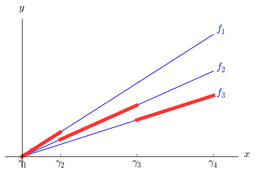
Let $y$ be a quantity (typically cost) that we wish to minimize. As before, we will assume that $y$ is a piecewise linear function of some variable $x$; for simplicity, I'll assume bounds $0 \le x \le U$ and $y\ge 0$. Let $0 = \gamma_1 < \cdots < \gamma_N < \gamma_{N+1}=U$ denote the breakpoints, and let $y=f_i(x)=\alpha_i x + \beta_i$ when $\gamma_i \le x < \gamma_{i+1}$, with the adjustment that the last interval is closed on the right ($f(U)=\alpha_N U + \beta_N$). With all units discounts, it is typical that the intercepts are all zero ($\beta_1 = \cdots = \beta_N = 0$) and cost ($y$) is proportional to volume ($x$), as seen in the first graph below, but we need not assume that. The second graph illustrates a somewhat more general case. In fact, we need not assume an economy of scale; the same modeling approach will work with a diseconomy of scale.

To model the discount, we need to know into which interval $x$ falls. Accordingly, we introduce binary variables $z_1,\ldots ,z_N$ and add the constraint $$\sum_{i=1}^N z_i = 1,$$ effectively making $\{z_1,\ldots , z_n\}$ an SOS1 set. Let $$M_i = \max_{0 \le x \le U} f_i(x)$$ for $i=1,\ldots,N$. Typically $M_i = f_i(U)$, but again we need not assume that. To connect the binary variables to $x$, we add for each $i\in \{1,\ldots,N\}$ the constraint $$\gamma_i z_i \le x \le \gamma_{i+1} z_i + U(1-z_i).$$ This just repeats the domain $0\le x \le U$ for all but the one index $i$ with $z_i = 1$; for that index, we get $\gamma_i \le x \le \gamma_{i+1}$.

The last piece is to relate the binary variables to $y$. We handle that by adding for each $i\in \{1,\ldots,N\}$ the constraint $$y\ge \alpha_i x + \beta_i - M_i(1-z_i).$$ For all but one index $i$ the right hand side reduces to $f_i(x)-M_i \le 0$. For the index $i$ corresponding to the interval containing $x$, we have $y\ge f_i(x)$. Since $y$ is being minimized, the solver will automatically set $y=f_i(x)$.

Adjustments for nonzero lower bounds for $x$ and $y$ are easy and left to the reader as an exercise. One last thing to note is that, while we can talk about semi-open intervals for $x$, in practice mathematical programs abhor regions that are not closed. If $x=\gamma_{i+1}$, then the solver has a choice between $z_i=1$ and $z_{i+1}=1$ and will choose whichever one gives the smaller value of $y$. This is consistent with typical all units discounts, where hitting a breakpoint exactly qualifies you for the lower price. If your particular problem requires that you pay the higher cost when you are sitting on a breakpoint, the model will break down. Unless you are willing to tolerate small gaps in the domain of $x$ (so that, for instance, the semi-open interval $[\gamma_i ,\gamma_{i+1})$ becomes $[\gamma_i , \gamma_{i+1}-\epsilon]$ and $x$ cannot fall in $(\gamma_{i+1}-\epsilon,\gamma_{i+1})$), you will have trouble modeling your problem.

LPs and the Positive Part

A question came up recently that can be cast in the following terms.  Let $x$ and $y$ be variables (or expressions), with $y$ unrestricted in sign.  How do we enforce the requirement that \[ x\le y^{+}=\max(y,0)\] (i.e., $x$ is bounded by the positive part of $y$) in a linear program?

To do so, we will need to introduce a binary variable $z$, and we will need lower ($L$) and upper ($U$) bounds on the value of $y$. Since the sign of $y$ is in doubt, presumably $L<0<U$.  We add the following constraints:\begin{align*} Lz & \le y\\ y & \le U(1-z)\\ x & \le y-Lz\\ x & \le U(1-z)\end{align*} Left to the reader as an exercise: $z=0$ implies that $0\le y \le U$ and $x \le y \le U$, while $z=1$ implies that $L \le y \le 0$ and $x \le 0 \le y-L$.

We are using the binary variable $z$ to select one of two portions of the feasible region.  Since feasible regions in mathematical programs need to be closed, it is frequently the case that the two regions will share some portion of their boundaries, and it is worth checking that at such points (where the value of the binary variable is uncertain) the formulation holds up. In this case, the regions correspond to $y\le 0$ and $y\ge 0$, the boundary is $y=0$, and it is comforting to note that if $y=0$ then $x\le 0$ regardless of the value of $z$.

OR and ... Parking??

'Tis the season to shop our brains out.  Two trips to a local mall today (neither, oddly enough, for the purpose of shopping) has me reflecting on the science (art?) of finding and selecting parking spots.  Choosing a parking spot involves elements of stochastic search (anyone have a link for this?), optimization of a distance function, and (when the mall is busy) stochastic stopping rules.

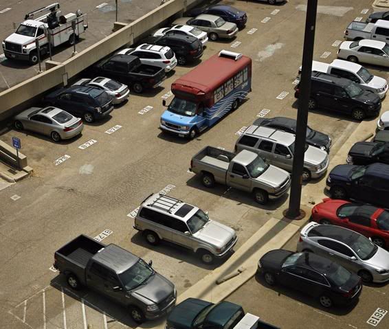
The application of stopping rules is fairly obvious, although the rule to use may not be.  You're running a search pattern through the packed parking lot of a mall, looking for an empty spot, when lo and behold you find one.  Now comes the stopping rule:  do you grab it, or do you continue the search, hoping for one closer to your immediate destination (the first store you plan to hit)?  If you pass it up and fail to find something closer, it likely will not be there the next time you go by.  Add an objective function that balances your patience (or lack thereof), your tolerance for walking, the cost of fuel, any time limits on your shopping spree and the possibility of ending up in a contest for the last spot with a fellow shopper possessing less holiday spirit (and possibly better armed than you), and you have the stopping problem.

The other obvious aspect is optimization of a distance metric, and this part tends to amuse me a bit.  Some people are very motivated to get the "perfect" spot, the one closest to their target.  My cousin exhibits that behavior (in her defense, because walking is painful), as did a lady I previously dated (for whom it was apparently a sport).  Parking lots generally are laid out in a rectilinear manner (parallel rows of spaces), and most shoppers seem to adhere rather strictly to the L1 or "taxicab" norm.  That's the appropriate norm for measuring driving distance between the parking spot and the store, but the appropriate norm for measuring walking distance is something between the L1 and L2 or Euclidean norm.  Euclidean norm is more relevant if either (a) the lot is largely empty or (b) you are willing to walk over (or jump over) parked cars (and can do so without expending too much additional energy).  Assuming some willingness to walk between parked cars, the shortest path from most spots to the store will be a zig-zag (cutting diagonally across some empty spots and lanes) that may, depending on circumstances, be closer to a geodesic in the taxicab geometry (favoring L1) or closer to a straight line (favoring L2).  The upshot of this is that while some drivers spend considerable time looking for the L1-optimal spot (and often waiting for the current occupant to surrender it), I can frequently find a spot further away in L1 but closer in L2 and get to the store faster and with less (or at least not much more) walking.

This leaves me with two concluding thoughts.  The first is that drivers may be handicapped by a failure to absorb basic geometry (specifically, that the set of spots at a certain Euclidean distance from the store will be a circular arc, not those in a certain row or column of the lot).  Since it was recently reported that bees can solve traveling salesman problems (which are much harder), I am forced to conclude that bees have a better educational system than we do, at least when it comes to math.  The second is that, given the obesity epidemic in the U.S., perhaps we should spend more time teaching algorithms for the longest path problem and less time on algorithms for the shortest path problem.

[Confession:  This post was motivated by the INFORMS December Blog Challenge -- because I thought there should be at least one post that did not involve pictures of food!]