Using Java Collections with CPLEX

Disclaimer: What follows is specific to Java, but with some name changes will also apply to C++. If you are using one of the other programming APIs for CPLEX, something analogous may exist, but I would have no idea about it.

I've seen a few questions by CPLEX users on forums recently that suggest the questioners may be moving from using a modeling language for optimization to using a general purpose language. Modeling languages tend to be more expressive (at least in my opinion) when it comes to writing optimization models. That's hardly shocking given that they are built for that purpose (and general programming languages are not). Recent questions have been along the lines of the following: I was using a structure (a tuple, or something similar) supported by the modeling language, and I don't know how to translate that to the general language; or I was creating arrays of variables / constraints / whatever indexed by something human-readable (probably names of things) and I don't know how to switch to integer-indexed arrays and keep it readable.

In my mind, the answer to those issues in Java is to make good use of classes and the Java Collection interface (and its various implementations). I'll give some examples in the context of a network flow problem.

In a modeling language, I might use a tuple to represent an arc. The tuple would consist of some identifier (string? index?) for the tail node of the arc, some identifier for the head node of the arc, and maybe an arc weight or some other arc property. In Java, I would create a class named Node to represent a single node, with fields including the node's name or other unique identifier and any costs, weights or other parameters associated with the node. Then I would create a class named Arc with fields of type Node holding the tail and head nodes, along with fields for any parameters associated with the arc (such as cost), and maybe a string field with a human-friendly label for the arc.

Now suppose I have an instance of IloCplex named cplex, and that I need a variable for each arc representing the flow on the arc. The conventional (?) approach would be to create a one dimensional array of IloNumVar instances, one per arc, and park the variables there. In fact, CPLEX has convenience methods for creating vectors of variables. The catch is that it may be hard to remember which index corresponds to which arc. One partial answer is to attach a label to each variable. The various methods in the CPLEX API for creating variables (and constraints) all have versions with a final string argument assigning a name to that variable or constraint. This works fine when you print out the model, but it's not terribly helpful while you're doing the coding.

I pretty much always use that feature to assign labels to variables and constraints, but I also employ collections in various ways. In my hypothetical network flow example, I would do something like the following.

HashSet<Node> nodes = new HashSet<>();
// Fill nodes with all node instances.
HashSet<Arc> arcs = new HashSet<>();
// Fill arcs with all arc instances.
HashMap<Arc, IloNumVar> flowVars = new HashMap<>();
HashMap<IloNumVar, Arc> flowArcs = new HashMap<>();
for (Arc a : arcs) {
  IloNumVar x = cplex.numVar(0, Double.MAX_VALUE, "Flow_" + a.getID());
  flowVars.put(a, x);
  flowArcs.put(x, a);
}

I put the nodes and arcs in separate collections (I used sets here, but you could equally well use lists), and then I create mappings between model constructs (in this case, arcs) and CPLEX constructs (in this case, variables). Collections can be iterated over, so there is no need to mess around with going back and forth between model constructs and integer indices. For each arc, I create a variable (and give it a name that includes the string identifier of the arc -- I'm assuming here that I gave the Arc class a getID method). I then map the arc to the variable and the variable to the arc. Why two maps? The arc to variable map lets me grab the correct variable while I'm building the model. For instance, a flow balance constraint would involve the flow variables for all arcs leading into and out of a node. I would identify all those arcs, park them in a collection (list or set), iterate over that collection of arcs, and for use the flowVars map to get the correct variables.

The reverse mapping I set up comes into play when the solver has a solution I want to inspect. I can fetch the value of each variable and map it to the corresponding variable, along the following lines.

HashMap<IloNumVar, Double> solution = new HashMap<>();
for (IloNumVar x : flowArcs.keySet()) {
  solution.put(x, cplex.getValue(x));
}

When I need to associate variable values with arcs, I can iterate over solution.entrySet(). For each entry e, flowArcs.get(e.getKey()) gives me the arc and e.getValue() gives me the flow on the arc.

Similar things can be done with constraints (IloRange instances).

Coordinating Variable Signs

Someone asked me today (or yesterday, depending on whose time zone you go by) how to force a group of variables in an optimization model to take the same sign (all nonpositive or all nonnegative). Assuming that all the variables are bounded, you just need one new binary variable and a few constraints.

Assume that the variables in question are $x_1,\dots,x_n$ and that they are all bounded, say $L_i \le x_i \le U_i$ for $i=1,\dots,n$. If we are going to allow variables to be either positive or negative, then clearly we need $L_i < 0 < U_i$. We introduce a new binary variable $y$ and, for each $i$, the constraints$$L_i (1-y) \le x_i \le U_i y.$$If $y$ takes the value 0, every original variable must be between its lower bound and 0 (so nonpositive). If $y$ takes the value 1, every original variable must be between 0 and its upper bound (so nonnegative).

Note that trying to enforce strictly positive or strictly negative rather than nonnegative or nonpositive is problematic, since optimization models abhor strict inequalities. The only work around I know is to change "strictly positive" to "greater than or equal to $\epsilon$" for some strictly positive $\epsilon$, which creates holes in the domains of the variables (making values between 0 and $\epsilon$ infeasible).

Minimizing a Median

\( \def\xorder#1{x_{\left(#1\right)}} \def\xset{\mathbb{X}} \def\xvec{\mathbf{x}} \)A somewhat odd (to me) question was asked on a forum recently. Assume that you have continuous variables $x_{1},\dots,x_{N}$ that are subject to some constraints. For simplicity, I'll just write $\xvec=(x_{1},\dots,x_{N})\in\xset$. I'm going to assume that $\xset$ is compact, and so in particular the $x_{i}$ are bounded. The questioner wanted to know how to model the problem of minimizing the median of the values $x_{1},\dots,x_{N}$. I don't know why that was the goal, but the formulation is mildly interesting and fairly straightforward, with one wrinkle.

The wrinkle has to do with whether $N$ is odd or even. Suppose that we sort the components of some solution $\xvec$, resulting in what is sometimes called the "order statistic": $\xorder 1\le\xorder 2\le\dots\xorder N$. For odd $N$, the median is $$\xorder{\frac{N+1}{2}}.$$For even $N$, it is usually defined as $$\left(\xorder{\frac{N}{2}}+\xorder{\frac{N}{2}+1}\right)/2.$$

The odd case is easier, so we'll start there. Introduce $N$ new binary variables $z_{1},\dots,z_{N}$ and a new continuous variable $y$, which represents the median $x$ value. The objective will be to minimize $y$. In addition to the constraint $\xvec\in\xset$, we use "big-M" constraints to force $y$ to be at least as large as half the sample (rounding "half" up). Those constraints are: \begin{align*} y & \ge x_{i}-M_{i}z_{i},\ i=1,\dots,N\\ \sum_{i=1}^{N}z_{i} & =\frac{N-1}{2} \end{align*} with the $M_{i}$ sufficiently large positive constants. The last constraint forces $z_{i}=0$ for exactly $\frac{N+1}{2}$ of the indices $i$, which in turn forces $y\ge x_{i}$ for $\frac{N+1}{2}$ of the $x_{i}$. Since the objective minimizes $y$, $z_{i}$ will be 0 for the $\frac{N+1}{2}$ smallest of the $x_{i}$ and $y$ will be no larger than the smallest of them. In other words, we are guaranteed that in the optimal solution $y=\xorder{\frac{N+1}{2}}$, i.e., it is the median of the optimal $\xvec$.

If $N$ is even and if we are going to use the standard definition of median, we need twice as many added variables (or at least that's the formulation that comes to mind). In addition to the $z_{i}$, let $w_{1},\dots,w_{N}$ also be binary variables, and replace $y$ with a pair of continuous variables $y_{1}$, $y_{2}$. The objective becomes minimization of their average $(y_{1}+y_{2})/2$ subject to the constraints \begin{align*} y_{1} & \ge x_{i}-M_{i}z_{i}\ \forall i\\ y_{2} & \ge x_{i}-M_{i}w_{i}\ \forall i\\ \sum_{i=1}^{N}z_{i} & =\frac{N}{2}-1\\ \sum_{i=1}^{N}w_{i} & =\frac{N}{2} \end{align*} where the $M_{i}$ are as before. The constraints force $y_{1}$ to be at least as large as $\frac{N}{2}+1$ of the $x_{i}$ and $y_{2}$ to be at least as large as $\frac{N}{2}$ of them. The minimum objective value will occur when $y_{1}=\xorder{\frac{N}{2}+1}$ and $y_{2}=\xorder{\frac{N}{2}}$.

Rolling Horizons

I keep seeing questions posted by people looking for help as they struggle to optimize linear programs (or, worse, integer linear programs) with tens of millions of variables. In my conscious mind, I know that commercial optimizers such as CPLEX allow models that large (at least if you have enough memory) and can often solve them (at least if you have enough computing resources to throw at the problems). My lizard brain, however, was conditioned by the state of the art in the late '70s to send me running (typically while screaming) at the sight of a model with more than, oh, 50 or so variables. Wrapping my head around tens of millions of variables, let alone thinking of a strategy for getting an optimal solution "quickly", is quite a struggle.

A former acquaintance from my student days once articulated his strategy for essay exams to me: if you don't know the answer, argue the premise of the question. In that vein, I'm inclined to ask why so many variables are necessary. One possibility is that the model captures decisions for a sequence of time periods. If decisions in one time period had no impact on subsequent periods, the problem would decompose naturally into a bunch of smaller problems; so if we are talking about a multiperiod model, it's safe to assume that the periods are connected.

That brings me to a strategy I learned back in primitive times, the "rolling horizon" approach. Let me stipulate up front that this is a heuristic method. It does not provide a provably optimal solution for the entire time horizon. Still, given the up-tick in humongous models, I'm starting to wonder if rolling horizons are no longer taught (or are looked down on).

The basic concept is simple. The devil is in the details. Let's say we want to solve a planning model over a horizon of $H$ time periods, and that one omnibus model for the entire horizon is proving intractable. The rolling horizon approach is as follows.

1. Pick a shorter horizon $K < H$ that is tractable, and a number of periods $F \le K$ to freeze.
2. Set "boundary conditions" (more on this below).
3. Solve a model for periods $1,\dots,K$, incorporating the boundary conditions.
4. Freeze the decisions for periods $1,\dots,F$.
5. Solve a model for periods $F+1,\dots, \min(F+K, H)$.
6. Repeat ad nauseam.

Note that if $F<K$, some decisions made in each solution but not frozen will be subject to revision in the next model.

The initial conditions (starting inventory, locations of vehicles, pending orders, ...) for each model are dictated by the state of the system after the last frozen period. The boundary conditions are limits on how much of a mess you can leave at the end of the reduced planning horizon (period $K$ in the first model, $K+F$ in the second model, etc.). More precisely, they limit the terminal state of things that will be initial conditions in the next model.

As a concrete example, consider a manufacturing scheduling model. You start with inventories of components and finished products, available capacity of various kinds, and unfilled orders, and you end with the same kinds of things. Without boundary conditions, your solution for the first model might end period $K$ with no finished goods inventory. Why make stuff if it doesn't count toward your demand within the time frame considered by the model? That might make the problem for periods $K+1$ onward infeasible, though: you have orders that must be filled, they exceed your immediate production capacity, and the cupboard was left bare by the previous solution.

So you want to add constraints of the form "don't leave me with less than this much inventory on hand" or "don't leave me with more than this many unfilled orders". Picking values for those limits is a bit of an art form. Make the limits too draconian and you will get a very suboptimal solution (say, piling up way more inventory than you'll really need) or possibly even make the early subproblems infeasible. Make the limits too laissez faire, and you may force thoroughly suboptimal solutions to later subproblems (piling on lots of expensive overtime, blowing off soon-to-be-former customers) or even make the later problems infeasible. Still, it's usually possible to come up with pretty reasonable boundary conditions, perhaps with some trial and error, and it's a way to get a solution that, if not globally optimal, is at least good (and preferable to staring bleary-eyed at your screen in the 30th hour of a run, wondering if the beast will ever converge).

The term "rolling horizon" was coined in reference to problems that are decomposed based on time, but the same concept may extent to problems that can be decomposed based on position. I used it not long ago to get a heuristic for a problem placing nodes in a physical network. In essence, we took the original geographic region and chopped it into pieces, picked a piece to start from, and then worked our way outward from that piece until all the pieces had been solved, each based on the (frozen) solution to the more inward pieces.

If This and That Then Whatever

I was asked a question that reduced to the following: if $x$, $y$ and $z$ are all binary variables, how do we handle (in an integer programming model) the requirement "if $x=1$ and $y=1$ then $z=1$"? In the absence of any constraints on $z$ when the antecedent is not true, this is very easy: add the constraint $$z \ge x + y - 1.$$Verification (by substituting all possible combinations of 0 and 1 for the variables) is left to the reader as an exercise.

I thought I had covered this in a previous post, but looking back it appears that it never came up (at least in this form). This might be my shortest post ever. :-)

Sharing "Implicit" Test Problems

The topic of reproducible research is garnering a lot of attention these days. I'm not sure there is a 100% agreed upon, specific, detailed definition of it, and I do think it's likely to be somewhat dependent on the type of research, but for purposes of this post the Wikipedia definition (previous link) works for me. In particular, I want to call out one part of the Wikipedia entry:

The term reproducible research refers to the idea that the ultimate product of academic research is the paper along with the laboratory notebooks and full computational environment used to produce the results in the paper such as the code, data, etc. that can be used to reproduce the results and create new work based on the research.

I've seen a lot of press related to reproducibility in the biological sciences, although I assume it's an issue in other sciences as well. (Good luck with that, physicists!) It's also increasingly an issue in the social sciences, where one study asserted that over half of the published results they tested failed to replicate. (That study itself was criticized as allegedly failing to replicate.) All of this has been termed by some a "replication crisis". In short, reproducibility is a big deal. There's at least one blog devoted to it, and a considerable amount of work in the statistics community is going into tools to facilitate reproducibility (such as R and Python "notebooks"). R users in particular should have a look at the rOpenSci Reproducibility Guide.

My research tends almost exclusively to fall into the category of "stupid math programming tricks". Either I'm trying to find some clever formulation of a (deterministic) problem, I'm trying to find an efficient way to generate an exact solution, I'm trying to find a decent heuristic for getting "good" solutions "quickly" (preferably without stretching analogies to nature too far: there's no way I'm beating slime mold optimization in the naming contest), or some combination of the above. Since I mostly avoid statistics (other than the occasional comparison of run times with some selected benchmark alternative), I've been largely unaffected by the debate on reproducibility ... until now.

Recently, the journals published by INFORMS have moved in the direction of reproducible research, and I suspect others are doing so (or will do so in the near future) as well. As an example relevant to my interests, the INFORMS Journal on Computing (JOC) has introduced policies on the sharing of both data and code. Personally, I think this is a good idea. I've shared data and code for one particular paper (machine scheduling) on my web site since the paper came out (20+ years ago), and I share data for a more recent paper as well (having released the code as an open source project).

At the same time, I recognize that there are various difficulties (licensing/copyright, for instance) in doing so, and also there are costs for the researcher. I'd be willing to share the code for one or two other projects, but it would take a major effort on my part to untangle the spaghetti and figure out which libraries are/are not required, and which code should be included or should be excluded as irrelevant to the ultimate experiments. I'm reluctant to commit that time until someone actually requests it.

There's another twist that I would not have anticipated until quite recently. I'm working on a project that involves "implicit hitting set" (IHS) problems. In an IHS problem, you have a master problem that formulates as a pure integer (in fact, 0-1) program. Candidate solutions to that model are fed to one or more "oracles", which either bless the solutions as feasible or generate additional constraints for the master problem that the candidates violate. Note that I have not said anything about the nature of the oracles. Oracles might be solving linear or integer programming models, which would be relatively easy to share as "data", but they might also be doing something decidedly funky that is encapsulated in their coding. In the latter case, the test "data" is actually code: I would have to provided the code for the oracles in order for someone to reproduce my results.

Well, okay, if sharing code is on the table now, isn't that just more code? Not quite. Let's say that some unfortunate doctoral student has been tasked by her advisor to code their shiny new IHS algorithm and test it against my published problems. The doctoral student used Python or Julia (or some other trendy language), whereas I used stodgy old Java, so there's a good chance the luckless doctoral student will have to recode my stuff (which, among other things, requires making sense of it). Moreover, I will have created an API to my oracles that may or may not fit with what they are doing ... and that's if I used an API at all. If I directly integrated program structures external to the oracle functions into the oracle (passed in variables, constraints or other elements of my master problems, for instance), our doctoral student will need to figure out how to isolate those elements and replace them with corresponding elements from her code ... if there is even a correspondence.

There's at least one implication in this for me. If I actually subscribe to the push for reproducibility (or if I take pity on other people's doctoral students), I need to code my oracles not as an integral part of my master code but as a separate software module or library with a well-documented and reasonably flexible interface to the outside world (API). <sigh>More work for me.</sigh>

Another Absolute Value Question

Someone asked whether it is possible to eliminate the absolute value from the constraint$$Lx\le |y| \le Ux$$(where $L\ge 0$ and $U>0$ are constants, $x$ is a binary variable, and $y$ is a continuous variable). The answer is yes, but what it takes depends on whether $L=0$ or $L>0$.

The easy case is when $L=0$. There are two possibilities for the domain of $y$: either $y\in [0,0]$ (if $x=0$) or $y\in [-U,U]$ (if $x=1$). One binary variable is enough to capture two choices, so we don't need any new variables. We just need to rewrite the constraint as$$-Ux\le y \le Ux.$$If $L>0$, then there are three possibilities for the domain of $y$: $[-U, -L] \cup [0,0] \cup [L, U]$. That means we'll need at least two binary variables to cover all choices. Rather than change the interpretation of $x$ (which may be used elsewhere in the questioner's model), I'll introduce two new binary variables ($z_1$ for the left interval and $z_2$ for the right interval) and link them to $x$ via $x=z_1+z_2$. That leads to the following constraints:$$-Uz_1 \le y \le -Lz_1 + U(1-z_1)$$and$$Lz_2 - U(1-z_2) \le y \le Uz_2.$$ If $x=0$, both $z_1$ and $z_2$ must be 0, and the new constraints force $y=0$. If $x=1$, then either $z_1=1$ or $z_2=1$ (but not both). Left to the reader as an exercise: verify that $z_1=1\implies -U\le y \le -L$ while $z_2=1 \implies L\le y\le U$.

MIP Models in R with OMPR

A number of R libraries now exist for formulating and solving various types of mathematical programs in R (or formulating them in R and solving them with external solvers). For a comprehensive listing, see the Optimization and Mathematical Programming task view on CRAN. I decided to experiment with Dirk Schumacher’s OMPR package for R. OMPR is a domain specific language for linear and mixed-integer linear programs. OMPR currently relies on the R Optimization Infrastructure package (ROI), which uses a plugin architecture to act as a bridge between R code and third party solvers (including CPLEX). The CPLEX plugin for ROI, in turn, has a dependency on the RCplex package to connect to CPLEX.

Of course, to try out an optimization modeling package you need to have something to optimize. I went back to some ancient research I did, specifically a paper in 1990 on using MIP models to choose linear (or polynomial) discriminant functions for classifying observations into one of two groups. For the sleep deprived, the full citation is:

Rubin, P. A. Heuristic solution procedures for a mixed-integer programming discriminant model. Managerial and Decision Economics, Vol. 11, No. 4, October 1990.

I used Anderson's iris data for the test case (since it's conveniently available in R, through the datasets package), and just for the halibut I also threw in a support vector machine (SVM) model using the kernlab package for R. Comparing the two is a bit misleading, since SVM models are inherently nonlinear, but I just felt like doing it. In any case, the purpose is to see how OMPR works with CPLEX, not to compare MIP discriminant models and SVMs.

The details are too lengthy for a blog post, so I posted them separately in an R notebook. If you're not familiar with R notebooks, you can find details here. The web page generated by my notebook contains the source code, and there's a control in the upper right of the web page that will let you download it as a notebook (R Markdown) file. You can also grab it from my GitLab repository for the project. As with other content of this blog, it's yours to play with under a Creative Commons license.

The MIP model is as follows. We start with samples of two classes ( "positive" and "negative") containing $p$ features. Let $X_1$ be the $N_1\times p$ matrix of data for the negative sample and let $X_2$ be the $N_2\times p$ matrix of data for the positive sample. The discriminant function we wish to train is $f(x)=w'x+c$; we will classify an observation $x$ as belonging to the positive or negative class according to the sign of $f(x)$. To allow for both limited measurement accuracy of the data and the inevitable adventures with rounding error, we arbitrarily choose some constant $\delta > 0$ and declare a positive observation correctly classified if $f(x)\ge \delta$ and a negative observation correctly classified if $f(x)\le -\delta$.

To avoid the pitfall of having the solver scale $w$ up to some ridiculous magnitude in order to force borderline observations to "look" correctly classified (i.e., to get around the use of $\delta$ as a minimum magnitude for non-zero classification scores), we bound $w$ via its sup norm: $-1 \le w_j \le 1 \, \forall j\in \{1,\dots,p\}$. The constant term $c$ is unbounded and unrestricted in sign.

To detect and count misclassifications (including ambiguous classifications, $-\delta < f(x) < \delta$, we introduce binary variables $y_i,\, i\in\{1,\dots,N_1\}$ for the negative sample and $z_i,\, i\in\{1,\dots,N_2\}$ for the positive sample. Each will take value 0 if the corresponding observation is correctly classified and 1 if not. In the OMPR demo, I just count total misclassifications ($\sum_i y_i + \sum_i z_i$); in general, misclassifications can be weighted to account for prior probabilities, oversampling of one group relative to the other, or relative importance of different types of errors (e.g., false positives looking for cancer tumors are bad, but false negatives can be fatal). There is also a variable $d$ that captures the minimum absolute value of any correct classification score (i.e., how far correct scores are from the boundary value of 0). Larger values are rewarded in the objective function (using a coefficient $\epsilon > 0$).

The model also contains "big M" type constraints to define the binary variables. Formulas for selecting the values of the parameters $M_1$, $M_2$ and $\epsilon$ are given in the paper. So, finally, we get to the MIP model:


\begin{alignat*}{2} & \textrm{minimize} & \mathbf{1}^{\prime}y+\mathbf{1}^{\prime}z-\epsilon d\\ & \textrm{subject to}\quad & X_{1}w+c \cdot \mathbf{1}+d \cdot \mathbf{1}-M_{1} \cdot y & \le 0\\ & & X_{2}w+c \cdot \mathbf{1}-d \cdot \mathbf{1}+M_{2} \cdot z & \ge 0\\ & & w & \le \mathbf{1}\\ & & w & \ge -\mathbf{1}\\ & & c \quad & \textrm{free}\\ & & d \quad & \ge \delta\\ & & y, \: z \quad & \textrm{binary} \end{alignat*}

Better Estimate, Worse Result

I thought I might use a few graphs to help explain an answer I posted on Quora recently. First, I'll repeat the question here:

In parametric optimization with unknown parameters, does a better estimator of the parameter always lead to better solutions to the actual problem?

Here we’re trying to minimize $f(x,\theta)$ with respect to $x$, but we don’t know the value of $\theta$. We may have several estimators of $\theta$, and we’re comparing them in a mean square error sense (or by some other loss function in general).

One would like to believe that better estimates lead to better answers, but the word "always" is a deal-breaker. Well, with one exception. The answer to the question is (trivially) yes if "better estimator" is interpreted to mean "estimator yielding better objective value". For mean square error or any other likely loss function, though, "better" is going to mean "closer to $\theta$" (in some sense of "closer"), and that's when things fall apart.

I'm going to take a couple of liberties in my answer. First, I'm going to change minimization of $f$ to maximization, just because it makes the pictures a little easier to interpret. Clearly that makes no meaningful difference. Second, I'm going to assume that maximization of $f$ is constrained. I can cobble together a similar but unconstrained counterexample by replacing the constraints with a penalty function (and assuming some bounds on the domain of $\theta$), but the constrained counterexample is (I think) easier to understand.

For my counterexample, I'll take a simple linear program in which the constraints are known with certainty but $\theta$ provides the objective coefficients:

$$\begin{array}{lrcl} \max & \theta_{x}x+\theta_{y}y\\ \text{s.t.} & x+y & \le & 3\\ & x & \le & 2\\ & y & \le & 2\\ & -x & \le & 0\\ & -y & \le & 0 \end{array}$$
I deliberately wrote the sign constraints $x \ge 0, y \ge 0$ "backwards" to fit Figure 1 below.

Figure 1

The feasible region is the polytope with vertices A, B, C, D and E. The dotted lines are (unit length) normals to the constraint hyperplanes. So $a^{(2)}$ is the coefficient vector (1, 1) of the first constraint, scaled to unit length, $a^{(5)}=(-1, 0)$ is the coefficient vector of the sign restriction on $x$ and so on. (I numbered the normals in clockwise order around the polytope, rather than in the order the constraints are written above.)

The red dashed vector represents a possible realization of the parameter $\theta$. Since we're maximize, $f$ increases in the direction that $\theta$ points, so for this particular realization vertex B is the unique optimum.

Note that $\theta$ in Figure 1 is between $a^{(1)}$ and $a^{2}$. This is not a coincidence. If $\theta$ is parallel to one of the constraint normals $a^{(j)}$, all points on the edge corresponding to that constraint will be optimal. If $\theta$ lies strictly between two constraint normals, the vertex where their edges intersect will be the unique optimum. This is easy to prove (but I won't bother proving it here).

Figure 2 shows this situation in the same two dimensional space. The five constraint normals divide the space into five circular cones, with each cone corresponding to a vertex. If $\theta$ lands in the interior of a cone, that vertex is optimal. If it falls on an edge between two cones, both the corresponding vertices (and all points along the edge between them) are optimal.

Figure 2

In Figure 2 I've drawn a particular realization of $\theta$ (deliberately not the one from Figure 1), and two estimators $\hat{\theta}$ and $\tilde{\theta}$. Unfortunately, I'm limited to raster image formats and not vector formats in the blog, so the plots get rather fuzzy if you zoom on them. You'll have to take my word for it that $\hat{\theta}$ is the black vector just above the negative $x$ axis and $\tilde{\theta}$ is the black vector just clockwise of the positive $y$ axis. Alternatively, you can click on the image and download it or open it. (The images have transparent backgrounds, so I recommend opening them in your browser, or some other application that will supply a background.)

By design, I've selected them so that $\tilde{\theta}$ is geometrically closer to $\theta$ than $\hat{\theta}$ is. That should make $\tilde{\theta}$ the better estimator of the two in terms of squared error, absolute deviation ($L_1$ error), etc. Unfortunately, using $\tilde{\theta}$ results in vertex B being the unique optimum. Using the true coefficient vector $\theta$, vertex A is optimal, and the seemingly inferior estimator $\hat{\theta}$ also falls in the cone where A is optimal.

Thus using the "inferior" estimator $\hat{\theta}$ gets you the correct answer, albeit with a somewhat incorrect prediction for the value of the objective function. Using the "superior" estimator $\tilde{\theta}$ gets you a flat-out suboptimal solution. In Figure 1, the incorrect solution B looks to be not too far (geometrically) from the correct solution A, but I could easily cook this example so that B is a long way from A, guaranteeing a massively incorrect result.

All that said, I would still gravitate to the more accurate estimator and not sweat the occasional pathological outcome. Sadly, though, there is once again no guarantee that doing the right thing leads to the best result.

Enforcing Simultaneous Arrivals

I'm recapping here an answer to a modeling question that I just posted on a help forum. (Since it will now appear in two different places, let's hope it's correct!)

The original poster (OP) was working on a routing model, in which vehicles (for which I will use $v$ and if needed $v'$ as indices) are assigned to visit customers (index $c$) at various (strictly positive) times. Different customers need different numbers of vehicles. We'll assume, for simplicity, that each customer is visited only once (or at most once, if you're allowed to blow off customers). If customers can be revisited, we can finesse it by creating clones of the customers (so $c$ and $c'$ are actually the same customer at different times).

I'll skip much of the formulation, which is irrelevant to the issue here. The problem confounding the OP was that if multiple vehicles serve the same customer, they must arrive at the same time. I suggested two ways to formulate this, described below.

Discrete time approach

Let's assume that the time frame (call it 0 to $T$) can be adequately approximated by a discrete sequence $$0=t_0 \lt t_1 \lt \dots \lt t_N=T.$$ Define a set of binary variables $x_{cvn}$ to be 1 if vehicle $v$ serves customer $c$ at time $t_n$ and 0 otherwise. To enforce the simultaneity requirement, we add the constraints $$x_{cvn} = x_{cv'n}$$for all combinations of $c$, $n$ and $v\neq v'$. The good news is that it's relatively easy to do and numerically stable. The bad news is that it requires a ton of binary variables ($C\times V\times N$, where $C$ is the number of  customers, $V$ the number of vehicles and $N$, as noted, the number of time epochs) and constraints ($C\times N \times \frac{V\times (V-1)}{2}$). The constraints could hypothetically be added "lazily" via callbacks, but I'm not sure that whether that would help or hurt performance.

Big $M$ approach

Let's stipulate, for convenience, that a vehicle is assigned arrival time 0 at a customer if the vehicle does not serve that customer. The alternative approach relies on the fact that the absolute difference between any two arrival times cannot exceed $T$. We can use a "big $M$" model with $T$ serving as our value for the infamous coefficient $M$.

Let $y_{cv}$ denote the time at which vehicle $v$ arrives at customer $c$ (or 0 if the assignment of $v$ to $c$ is not made). The $y$ variables can be considered continuous, and we do not need to discretize time. We will also need binary variables $z_{cv}$ taking the value 1 if vehicle $v$ services customer $c$ and 0 if not. We add the constraints $$y_{cv}-y_{cv'} \le T(2 - z_{cv} - z_{cv'})$$and $$y_{cv'}-y_{cv} \le T(2 - z_{cv} - z_{cv'})$$for all combinations of $c$ and $v\neq v'$. We'll also need constraints to tie $y$ and $z$ together, namely $$y_{cv}\le Tz_{cv}$$for all combinations of $c$ and $v$. If serving a customer at time 0 is not legal, and $\tau \gt 0$ is the earliest possible service time, throw in$$y_{cv}\ge \tau z_{cv}$$for all $c, v$ pairs. Using the previous notation, this requires $C\times V$ binary variables (the continuous variables are harmless) and at worst $C\times V\times (V-1)+2\times C\times V$ constraints, which is considerably more compact than the previous approach. Two possible downsides -- the only ones I see off the top of my head -- are that if $T$ is large, it may create numerical stability issues and/or cause LP relaxations to be loose (for both of which "big $M$" models are infamous).

Using CLP with Java

The COIN-OR project provides a home to a number of open source software projects useful in operations research, primarily optimization programs and libraries. Possibly the most "senior" of these projects is CLP, a single-threaded linear program solver. Quoting the project description:

CLP is a high quality open-source LP solver. Its main strengths are its Dual and Primal Simplex algorithms. It also has a barrier algorithm for Linear and Quadratic objectives. There are limited facilities for Nonlinear and Quadratic objectives using the Simplex algorithm. It is available as a library and as a standalone solver. It was written by John Forrest, jjforre at us.ibm.com.

Like most of the projects at COIN-OR, CLP is coded in C++, which can make it a bit of a pain to use from Java. So I was quite interested when Nils Löhndorf wrote to me that he had written a Java interface to CLP, clp-java, which he has released as open source. I have an academic license for CPLEX, so I'm not really motivated to switch to CLP, but in the past I've found myself working on open source projects in which I would like to have embedded an LP solver. Since the intent is that people be able to use the program at no cost, embedding a somewhat expensive commercial solver is clearly a non-starter.

So I downloaded clp-java and took it for a test drive. I coded a basic assignment model in Java, with randomly generated assignment costs and a user-selectable dimension. (By "dimension" I mean number of slots and number of assignees.) Each run solves a single assignment problem twice, once with CLP and once with CPLEX. Since CLP is limited to a single thread, I throttled CPLEX to a single thread as well.

My primary objective was not to see which was faster. Hans Mittelmann at Arizona State University maintains solver benchmarks in his Decision Tree for Optimization Software. You can see there that CLP sometimes beats CPLEX (rather handily) but frequently is slower. (The same can be said for CLP in comparison to Gurobi.) What I wanted to know was the following:

• is clp-java easy to use (yes!) and well-documented (pretty well);
• does it produce correct answers (yes, at least on my tests -- CLP and CPLEX obtained identical solutions on all tests);
• is there any performance penalty for using the clp-java interface (not that I can see).

I started with a dimension of 5 and doubled it with each new run, up to 1280 for the final run. Here's a log-log plot of total end-to-end solution times:

CPLEX beat CLP consistently, but as problem dimension grew the ratio of times seemed fairly steady, and the difference (a bit over 25 seconds on my quad-core PC) doesn't strike me as horrible. IMPORTANT DISCLAIMER: We're looking at one replication at each problem size of one particular LP (assignment problem). Ascribe any significance to anything I say at your own peril. Also, I repeated a few replications, and the times varied significantly, even though the seed for the random number generator was held constant (meaning the repeated problems should have been identical to the original versions). So the teeny sample size is exacerbated by fairly high variance.

I broke the timing down into three parts: setting up the model; solving the model; and recovering the solution (getting the solver to cough up the values of the assignment variables). Here are log-log plots for each.

Setup

CPLEX seemed to be a bit faster creating a model object than CLP was, but the difference was pretty minimal (2.3 seconds with 1,280 assignees).

Solution

The bulk of the time for either program is spent solving the problem, so this plot resembles the plot of overall execution times.

Recovery

For the small models, both program returned the variables values so quickly that the recorded time (in milliseconds) was zero. Interestingly (at least to me), on the larger instances CLP returned solution values faster than did CPLEX.

Again, the takeaway from the experiments is not which solver is better; it's that Nils's interface works correctly and does not seem to introduce any glaring inefficiencies. Overall, I am quite impressed with Nils's creation. He provides an all-in-one jar file that contains not only his code but also CLP and some third-party libraries. You only have to import clp-java into your project and put the jar in the class path. When you run your program, the necessary libraries are unpacked into a temporary directory. Before the program exits, it cleans up after itself, deleting the temporary directory. (I confirmed that it left no digital artifacts behind.)

There is one bug yet to be worked out (as of this writing). At least on Ubuntu 14.04 and Linux Mint 17.2 (based on Ubuntu 14.04), "out of the box" you get linking errors at run time. Apparently, despite the fact that the COIN libraries CLP uses are sitting in the same temporary directory that CLP is sitting in, it looks for them elsewhere and can't find them. The workaround is to install the coinor-clp package (and a couple of dependencies) from the Canonical repositories, using apt or Synaptic. That fixed the linking problem for me and one other user. I have no idea if the same problem crops up in other operating systems.

So if you are programming in Java and looking for an open-source LP solver that you can build into a project, check out clp-java and CLP.

Rounding Error

I recently experienced the eight-bazillionth iteration of the following scenario. Someone posts a request for help on a forum. They are doing some sort of MIP model, or possibly something even more advanced (Benders decomposition, column generation, ...), and things are not going well. In some cases they think they have made a coding error; more commonly they think the solver (CPLEX in my personal experience, since that's the only one whose forums I watch) has a bug in it. After substantial back and forth, the key problem emerges: their binary variable came out 1.00000 E-9 or 0.99999999, which is "clearly" neither 0 nor 1.

At this point, my reaction is always the same (add your favorite expletives after every few words): "Don't they know about rounding error???"

In fairness, though, they may not, and perhaps the blame lies on the shoulders of faculty (possibly including me, in my former life). One of the courses I took during my first term of graduate school (in math) was numerical analysis. This is back when mainframes were just making the transition from vacuum tubes to semiconductors, and "user input" was a euphemism for "deck of punch cards". It's also a time when memory was at a premium and, thus, single precision ruled the realm.

(BEGIN TANGENT) I suspect that some readers who are (much) younger than I, and who program, will have noticed that pretty much everything of a floating point nature is automatically done double-precision these days, and may be wondering why single-precision float types still exist. They're a holdover from my youth, and I suspect exist almost exclusively for backward compatibility. (END TANGENT)

I don't recall why I picked numerical analysis as an elective -- whimsy, I think -- but it ended up being one of the most useful courses I took in grad school. The first, and most important, lesson from it was that computers do math inexactly. This should be immediately obvious if you stop to think about it. I learned in childhood that 0.3333... = 1/3, where the ... means "repeated an infinite number of times". Stop the decimal expansion after a finite number of digits, and you get something slightly less than 1/3. Now pretend for the moment that your computer encoded numbers in decimal rather than binary, and that you used the expression 1/3 in a program. The compiler would convert 1/3 to a decimal representation, but not 0.3333... -- because that would require an infinite amount of memory to store, and the computer only has a finite amount. So the computer has to truncate the decimal expansion, and as a result what the computer stores for 1/3 is not actually 1/3. (Now go back to using binary. The same logic applies.)

I'm not going to repeat an entire course in numerical analysis here (too much typing), but another lesson I learned was that, when programming, I should never do strict equality comparisons on anything that was not stored as an integer. Here's a small example that I just ran in R (not to pick on R -- it was just handy):

> sqrt(9) - 2.99999999999999999 == 0
[1] TRUE

To a mathematician, that relation is patently false, but to the program the decimal expansion is "close enough" to 3.

My prof shared one anecdote that has stuck with me for almost half a century now. He told of an engineer who coded his own routine for inverting a matrix and was not particularly careful about dealing with rounding errors (and "stiff" matrices, a topic for another time). The engineer then published a paper which included, at one point, the inverse of a particular matrix, computed by his program, with each entry in the matrix printed to some absurd number of decimal places (five, I think). All the digits to the right of the decimal points were wrong. So were the first couple of digits immediately left of the decimal points. You can ignore the limitations of computer arithmetic precision, but (queue sinister background music) those limitations will not ignore you.

Where I'm going with this is that I learned about the limitations of computer math somewhat accidentally, because I just happened to take numerical analysis. I suspect that some OR/IE programs require it, and I'm pretty sure others (most?) don't. In the interests of reducing frustration for a lot of people (of whom I'm the only one I care about), and perhaps avoiding incorrect results being published, I think we should pressure anyone teaching computational topics in OR (particularly, but not exclusively, integer programming) to provide some minimal coverage of rounding and truncation errors, the IEEE standards for single- and double-precision values, etc. If they cannot (or will not) teach it themselves, they can at least require that the student go learn it as a prerequisite.

Please! I'm begging you!

Matching Ordering Is Not Always Easy

In some circumstances, you might want to build an optimization model containing two sets of variables, say $x_1,\dots,x_N$ and $y_1,\dots,y_N$, and constrain them so that the sort order of each matches. That condition is easily expressed in logical terms: $x_i \ge x_j$ if and only if $y_i \ge y_j$ for all pairs $i,j \in \{1,\dots,N\}$ with $i\neq j$. Translating that into a mathematical programming model that is easy to solve may be tricky, though.

I'm thinking specifically of situations where you want your model to be a linear program or, at worst, an integer linear program. It is well known that linear programs have convex feasible regions, and that is the basis for most algorithms. For integer or mixed integer problems, solvers again rely on convexity, in two respects: the continuous relaxation of the model (relaxing integrality constraints) should have a convex feasible region; and the restricted problem obtained by fixing values for the integer variables should have a convex feasible region.

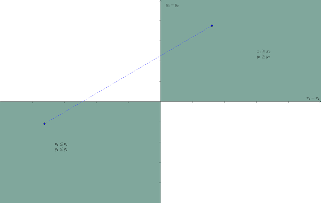
What makes the order matching constraint tricky can be seen in Figure 1 below. Let's assume for simplicity that $N=2$. Figure 1 shows a two dimensional space spanned by $x_1 - x_2$ and $y_1 - y_2$, with the set of points satisfying the ordering constraint (the first and third quadrants) shaded green. If we relax any integrality restrictions in the original model and project its feasible region (linearly) onto this plane, the "shadow" of the feasible region must lie within the green area.

Figure 1

Assuming the original feasible region (again, with any integrality restrictions relaxed) is convex, the way we want (need?) it to be, its projection will also be convex. The green area, though is not convex. The blue dotted line segment connects two feasible points but obviously leaves the green region. When we "cut away" the portion of the original feasible region that projects onto the white areas, we gain enforcement of the ordering constraint but may lose convexity of the feasible region.

So, are we screwed (to use a technical term)? Not necessarily. The projection of the original feasible region is unlikely to fill the green quadrants, and other constraints may cooperate to force the projection to remain convex. Figure 2 shows a somewhat trivial case, in which the original model also contains the constraint $x_1 - x_2 = y_1 - y_2$. That constraint by itself will cause the ordering restriction to be satisfied. The projection of the feasible region is the red line in Figure 2, which is clearly convex.

Figure 2

The takeaway from Figure 1, at least for me, is that getting the ordering constraint in while preserving convexity will be tricky in general (unless you get "lucky" courtesy of other constraints). Since the green area is the union of two convex sets (cones, to be specific), a standard way to finesse the convexity issue is to add a binary variable indicating which cone you are in. (See, for instance, Partitioning with Binary Variables.) Once the value of the binary variable is fixed, the feasible region is restricted to a particular quadrant (cone), and you can stop worrying about loss of convexity. You need a binary variable for each pair of subscripts, though, so in the general case this introduces $O(N^2)$ binary variables, which might get a bit annoying.

If all the variables are bounded and either $x$ or $y$ is integer valued, there might be a less cumbersome way to handle the ordering constraint, but that's a topic for another day (or never, whichever comes second).

Optimizing Part of the Objective Function II

Today's post extends yesterday's entry about optimizing a portion of the original objective function. I won't repeat much of the previous post, to save myself some typing.

The actual question motivating these posts, which I originally misread, asked how to minimize, not maximize, the sum of the $K$ largest terms in $\sum_{i=1}^N x_i$ (where $x$ is a vector of decision variables in an optimization model). As I mentioned in the last outing, that (or the symmetric case, maximizing the sum of the $K$ smallest terms), is trickier than what I covered yesterday. Everything from yesterday's post (the introduction of binary variables $z_i$ and auxiliary variables $y_i$ and the added constraints) carries over, with one exception: the objective function is now$$\textrm{minimize} \sum_{i=1}^N y_i.$$On top of all that, we require some additional constraints.

Update

Forget everything that follows and just skip down to the comments section. There's a clever reformulation, posted by Michael Grant in a comment, that gets the job done with a linear number of new variables (all continuous) and a linear number of constraints. I knew another formulation with no integer variables, and in fact only one new variable at all, but with an exponential number of constraints. I was debating whether to post it until I saw the more efficient solution in Michael's comment.

5. Lower bounds on auxiliary variables

If we do not do something to prevent it, the solver will achieve an ideal objective value of 0 by setting $y_i = 0$ regardless of whether $z_i$ is 0 or 1. So we need additional constraints to ensure that $z_i = 1 \implies y_i = x_i$. We can accomplish that with$$y_i \ge x_i - U_i(1 - z_i)\quad \forall i \in \{1,\dots,N\},$$which forces $y_i\ge x_i$ if $z_i = 1$ and is vacuous if $z_i = 0$.

6. Choosing the $K$ largest terms

Choosing the largest of the $x_i$ was automatic when the objective was to maximize the sum. When the objective is minimization, the solver will "want" to choose the smallest of the $x_i$, and we need to constrain it to select the largest values. An easy way to do this is to note that choosing the $K$ largest values is equivalent to saying that every value chosen is at least as big as every value not chosen. Expressed mathematically,$$z_i = 1 \bigwedge z_j = 0 \implies x_i \ge x_j.$$Note that, having assumed $0\le x_k \le U_k\,\forall k$, the most negative that any difference $x_i - x_j$ could be would be $0 - U_j = -U_j$. That leads to the following additional constraints:$$x_i - x_j \ge -U_j(1-z_i+z_j)\quad \forall i,j\in \{1,\dots,N\},\,i\neq j.$$
Coupled with yesterday's formulation, that should get the job done.

Optimizing Part of the Objective Function

A somewhat curious question showed up on a forum today. The author of the question has an optimization model (I'll assume it is either a linear program or mixed integer linear program) of the form \begin{alignat*}{2} & \textrm{maximize} & & \sum_{i=1}^{N}x_{i}\\ & \textrm{s.t.} & & x\in\mathcal{X} \end{alignat*} where the feasible region $\mathcal{X}$ is presumably polyhedral. What the author wants to do is instead maximize the sum of the $K$ largest terms in the objective, for some fixed $K<N$. The question was how to do this.

In effect, the author wants to selectively turn some terms on and others off in the objective function. Any time I think about turning things on and off, I immediately think of using binary variables as the "switches". That in turn suggests the likely need for auxiliary variables and the very likely need for a priori bounds on the things being turned on and off. Here is one solution, step by step, assuming that the $x$ variables are nonnegative and that we know a finite upper bound $U_i$ for each $x_i$.

1. Introduce a binary variable for each term to be switched on/off.

So we add variables $z_i \in \{0,1\}$ for $i\in 1\dots N$, with $z_i=1$ if and only if $x_i$ is to be counted.

2. Limit the number of terms to count.

This is just the constraint $$\sum_{i=1}^N z_i = K$$ (with the option to change the equality to $\le$ if you want up to $K$ terms counted.

3. Replace the objective terms with surrogates that can be turned on/off.

We will add real variables $y_1,\dots,y_N$ and make the objective $$\textrm{maximize} \sum_{i=1}^N y_i.$$

4. Connect the surrogate variables to the original variables and the on-off decisions.

Here we benefit from a key property: if we limit the objective function to $K$ terms, the fact that we are maximizing will naturally favor the $K$ largest terms. So we just need the following constraints: \begin{alignat*}{2} y_{i} & \le x_{i} & & \forall i\in\left\{ 1,\dots,N\right\} \\ y_{i} & \le U_{i}z_{i} & \quad & \forall i\in\left\{ 1,\dots,N\right\} . \end{alignat*}If $z_i = 0$, the second constraint will force $y_i=0$ and the term will not contribute to the objective function. If $z_i=1$, the second constraint will become vacuous and the first term will allow $y_i$ to contribute an amount up to $x_i$ to the objective. Since the objective is being maximized, $y_i=x_i$ is certain to occur.

A symmetric version of this will work to minimize the sum of the $K$ smallest terms in the objective. Minimizing the sum of the largest terms or maximizing the sum of the smallest terms is a bit trickier, requiring some extra constraints to enforce $y_i=x_i$ when $z_i = 1$. Oops! It's actually easier, as pointed out in a comment in my next post.

Selecting the Least Qualifying Index

Something along the following lines cropped up recently, regarding a discrete optimization model. Suppose that we have a collection of binary variables $x_i \in B, \, i \in 1,\dots,N$ in an optimization model, where $B=\{0, 1\}$. The values of the $x_i$ will of course be dictated by the combination of the constraints and objective function. Now suppose further that we want to identify the smallest index $i$ for which $x_i = 1$ for use within the model (hence before solving the model). I'll consider two possibilities:

1. we want to store that minimal index in an integer variable (which I will call $z$); or
2. we want to create an alternative set of binary variables ($y_i \in B, \, i \in 1,\dots,N$) where \[ y_{i}=1\iff i=\text{argmin}\left\{ j:x_{j}=1\right\}. \]

I'll focus on the second case, which is a stepping stone to the first case. Once we have $y$ defined as in the second case, $z = \sum_{i=1}^n i y_i$ solves the first case.

To handle the second case, we can add the following constraints: \begin{alignat*}{2}
y_{i} & \le x_{i} & \; & \forall i\\
y_{i} & \ge x_{i}-\sum_{j<i}x_{j} &  & \forall i\\
iy_{i} & \le i-\sum_{j<i}x_{j} &  & \forall i>1
\end{alignat*}Left to the reader as an exercise: to confirm that this works (or, if you find an error, to kindly post it in a comment).

CPLEX Performance Variability

It may come as a surprise to some users of CPLEX that its performance is, somewhat intentionally, random. (This may be true of some other optimization software as well. I'll limit the assertion to CPLEX because CPLEX is the only solver for which I have first-hand knowledge that it's true.)

A certain amount of uncertainty about performance is probably inevitable. Operating systems swap programs in and out of memory and processes in and out of CPU cores in ways uncontrollable by the CPLEX user, so "random" fluctuations in timing are to be expected even when running code with identical parameter settings repeatedly on a single problem on a single machine. When the code is itself multi-threaded, I suspect even more "random" timing issues occur. (CPLEX by default uses multiple threads, but can be restricted to a single thread via a parameter setting.)

Less well known is that CPLEX uses a pseudorandom number stream to control some of its internal decision-making. Marc-André Carle (@ORNinja) has an excellent series of posts on his blog about performance variability, so I'll save myself a ton of typing and refer you there:

• Performance variability defined
• Performance variability: good readings
• Performance variability: consequences

I thought I'd share some recent results that demonstrate how one particular source of variability, the random seed, can make a large difference in performance. The name for the seed in the Java API is IloCplex.Param.RandomSeed. According to the CPLEX 12.6.1 parameters manual, its default value changes with each new release of the program, so if you run two different versions of CPLEX on the same problem, you can expect different performance even if none of the changes from one version to the next directly impact your problem. Put another way, your mileage WILL vary.

Here's an example. I took a moderately chewy MIP model that arises in a current research project. I'm not at liberty (nor inclined) to give a full description, but the first few lines of the CPLEX log show that it has what are, by contemporary standards, modest dimensions.

Reduced MIP has 20434 rows, 10239 columns, and 78243 nonzeros.
Reduced MIP has 215 binaries, 0 generals, 0 SOSs, and 0 indicators.
Presolve time = 0.08 sec. (37.97 ticks)
Found incumbent of value 216.000000 after 0.23 sec. (89.01 ticks)

This is a cost minimization problem with an integer-valued objective function. The trivial feasible solution with cost 216 is always found immediately; it's from there that the adventure begins. This version of the problem is not too difficult. Although I have not solved it to optimality yet, I'm fairly confident that the optimal solution has cost 11, and I suspect that a few hours of crunching on my quad-core PC would be enough to prove that solution is optimal.

I did a little test, using CPLEX 12.6.1, in which I did 85 independent solves, using different values of the seed parameter. Runs were limited to 60 seconds each and three CPU threads, and the Emphasis.MIP parameter was set to 4 (emphasizing a search for hidden feasible solutions -- improving incumbents -- over moving the lower bound or proving optimality). In other words, I told CPLEX to find good solutions fast, and to worry about proving optimality later. All other CPLEX parameters were left at default.

Here is a histogram of the lower bounds from those 85 runs:

The bounds ranged from 9.38 to 9.60, and you can see that the vast majority were at the low (inferior) end of the range. Now for a tabulation of the incumbents found within one minute:

Incumbent	11	12	144
Frequency	1	3	81

Recall that I am fairly certain the optimal value is 11. Out of 85 attempts, I landed on the optimal solution once and a near-optimal solution three times; on the other 81 tries, I got a fairly terrible solution (costing more than 13 times the optimum). There are some intermediate solutions with costs in the 20s and 30s that show up in the node logs for the runs where I got lucky; CPLEX just never happened to be sitting on one of those when the time limit expired.

The point here is that, in practice, users don't run the same problem multiple times with different seeds (if they even know the seed parameter exists, which I suspect most do not). This caught my eye because I'd done a test run on this example, gotten the incumbent down from 216 to 144 (with a lower bound under 10) after a minute or so, and thought "hmm, this is going to take a while". I might add that 144 was found fairly quickly, so there was a lengthy stretch with no progress in the incumbent before time ran out. Had I been lucky on that pilot run (where, if the table is to be believed, being lucky has probability a bit under 1 in 20), I would have gotten a really good solution (11 or 12) in the first minute, with a lower bound of 10 (rounding up, since the objective is integer-valued), and thought "hmm, this problem is pretty easy".

So, is the problem easy or not? Beats me.

I'll finish this with a pointer to a slide in a recent present on advances in CPLEX. The slide mentions a "racing ramp-up phase" that can be used when running CPLEX on multiple processors in parallel. In essence, CPLEX tackles the same problem independently on multiple processors, using different parameter settings for each. After a set amount of time (the end of the "ramp-up" phase), the results are compared, a winner is declared, and the processors then all proceed to work on finishing the winner's search tree, using the winner's parameter settings.

With or without parallel processors, a user can replicate this to some extent. In particular, you can do a set of short runs with different seeds, find the best incumbent solution found by any of them, restart with that seed and do a full production run. I don't think there's a way to recycle the winner's search tree (unless you get lucky and the last run was the winner, in which case you can just continue it), but if the ramp-up phase is kept short, this could still help.

Bottom line: a "hard" problem might be truly hard (CPLEX will take a long time no matter seed you use), or it might be hard in the sense that there are (many) more bad seeds than good. Then again, maybe you just need better karma.

Formulating Optimization Models

Periodically, on OR Exchange and other forums, I encounter what are surely homework problems involving the construction of optimization models. "The Acme Anvil Corporation makes two types of anvils, blue ones and red ones. Blue anvil use 185 kg. of steel and have a gross revenue of $325 each; red anvils ..." Really? Does anyone seriously believe Acme Anvil uses metric units?? This is obviously a homework problem.

Not surprisingly, these sorts of questions tend not to get answered, or at least not fully. Many of the participants in the forums are academics (faculty or students) who are loathe to corrupt the homework process; most of the rest have real jobs, and better things to do than other people's homework. Still, there's something to be said for providing some nonspecific guidance on how a student might get started formulating such a model.

After bumping into one on a forum earlier today, it occurred to me to post here, somewhat paraphrased and highly condensed, my "introduction to modeling" lecture from the Dark Ages, when I taught modeling to business students. A caveat is in order: this is for beginners in the modeling process. Experienced modelers will go through these steps implicitly/subconsciously/automatically or perhaps just dive straight into a relevant model by association with previously encountered models.

In essence, what follows is a checklist for formulating an optimization model. For whatever it's worth, here it goes.

Variables: Identify your decisions.

An optimization model is typically a decision-making model. Rather than attempting to go from first reading of the problem to full-fledged algebraic formulation, start by identifying the key decisions you must make (e.g., how many red anvils to make in March at the Los Alamos plant). Each decision maps to a single variable in your model. You will not necessarily come up with all the variables at this step, but you should identify the important ones. It might be helpful to think of yourself as the supervisor of some diligent but not very bright (and thoroughly non-quantitative) employees. (Think Harvard MBAs here.) What orders would you need to give them to get things running properly? Those are at least some of your decisions/variables.

As you identify decisions, also select units for them. Are anvils produced individually or in pallets? Is paint ordered by the gallon, by the thousand gallons, by the jug ...? Also ask yourself whether the amounts are continuous or discrete. Time spent on something is pretty continuous. Number of anvils produced is rather discrete.

Since discrete variables generally make models harder to solve, you might ask whether it's reasonable to treat seemingly discrete amounts a continuous. One example I used for this is the manufacture of ball bearings. The little buggers are obviously discrete -- nobody uses 4.37 ball bearings in the manufacture of a device -- but you probably make the little guys by the rail carload. If you decide to make 2.134 carloads today, nobody's going to obsess about whether that translates to a partial ball bearing.

My classroom experience suggests that this step is critical. Almost every time I had a student foundering in an attempt to formulate a model, their difficulty traced back to incorrect identification of the decision variables.

Bounds: What are reasonable values for your decisions?

The question here is not what specific values do you want; that's the solution to the model. The question is, in general terms, how big or small can each decision quantity be? The answers give upper and lower bounds for your decision variables. Often the lower bound will be zero, signaling that (a) you are measuring things the way most people do (negative quantities are inherently unnatural for most people) and (b) you might possibly not want to do whatever this variable represents at all. Upper bounds do not need to be very tight, and definitely should not be too tight (too tight meaning it cuts off a valid decision that might prove to be optimal). How many red anvils might I choose to make in a day? Without getting mired in resource issues, simple logic might suggest that more than 1,000 is out of the question. So I can use 1,000 as the upper bound for that quantity.

Objective function: What is my criterion for selecting a program of action?

Suppose that some intern came to you with several choices for what to do (how many anvils of each type to make, how many to put into storage, which ones to drop off cliffs, ...). How would you decide which solution was best? The criterion you use will turn into your objective function. Common choices include maximizing profit or minimizing cost (or, if you're the government, maximizing cost), but it could be something non-monetary such as maximizing the number of at-risk subjects inoculated against some disease or maximizing the amount of food aid distributed to a stricken area.

Having determined your decision criterion, you need to express it as a function (preferably linear, but life isn't always cooperative) of your decision variables. In attempting to do so, you may identify quantities other than decision variables that you need to know (or that would be helpful) in order to express the objective function. Those quantities will turn into auxiliary variables. Mathematically, there's no difference between a "decision" variable and an "auxiliary" variable; the distinction is largely in whether it looks like something you would decide explicitly (previous section) or implicitly (this section).

A common example of an auxiliary variable for business students is inventory. How many blue anvils should be put into inventory in March to be shipped in April? You might not have thought of that as an explicit decision when identifying the original variables. When you try to express profit (your criterion) as a function, however, you realize that there are costs for carrying inventory, and you must account for them ... which requires knowing how much inventory you have. Thus are born the inventory variables.

There are methods for handling multiple competing criteria (I want to maximize distribution of food aid while minimizing the cost of acquiring and distributing it), but beginners are urged to start with a single criterion. If you must account for multiple criteria, you will need to do one or more of the following:

• prioritize them;
• set reasonable targets (aspiration levels) for them;
• weight them (e.g., I'm indifferent between feeding one more person and saving $20 in cost).

Constraints: What restricts your decisions?

At this juncture, the ideal set of decisions is likely to be obvious. Make an infinite number of anvils and sell them all for a profit (at the risk of causing road runner extinction). Eat as much as you want of all the foods you like. Sadly, various factors will constrain your free will here. There's only so much iron available for anvils, your factories have limited capacity, and demand for anvils is not infinite. Your wallet will not support that all-steak diet, your wardrobe will not support the change in dimensions resulting from all the ice cream you can eat, and your doctor (or mother) (or both) absolutely insists that something green is mandatory (and mint ice cream does not qualify).

Your task now is to identify the aspects of the situation that will limit your decisions and express them as equations or inequalities involving your decision variables. Again, you may identify auxiliary variables during this process. If you do not have a specific accounting cost for holding inventory, you might not have identified it in the previous section. When it comes time to connect anvil production with anvil shipments, though, you may find it convenient to create inventory variables.

For strictly mathematical reasons, you will need to avoid strict inequalities. Where quantities are discrete, this is easy. "I need to make more than 50 blue anvils" (strict inequality, verboten) is equivalent to "I need to make at least 51 blue anvils" (weak inequality, perfectly legal). In other cases, it may not be so easy. "We need to make some blue paint" sounds a lot like "blue paint production $> 0$", but that's a strict inequality. Your choices are either "blue paint production $\ge 0$" (allowing the possibility that you produce no blue paint) or "blue paint production $\ge \epsilon$ where $\epsilon$ is a strictly positive parameter (a lower production limit that is the minimum amount you can live with).

I hope someone finds that helpful.

Partitioning with Binary Variables

Armed with the contents of my last two posts ("The Geometry of a Linear Program", "Branching Partitions the Feasible Region"), I think I'm ready to get to the question that motivated all this. Let me quickly enumerate a few key take-aways from those posts:

• The branch and bound method for solving an integer linear program or mixed integer linear program uses a search tree.
• At each node of the search tree, a linear program (LP) that relaxes some or all of the integrality restrictions (while adding some new restrictions based on earlier branching) is solved. (As an aside, this hold for mixed integer quadratic programs, with the change that the node relaxation will likely be a quadratic program rather than a linear program.)
• LPs have closed and convex feasible regions.
• The act of branching (separating a node into two child nodes) partitions the feasible region for the problem at the parent node into two smaller feasible regions.

Let's move on now. A common use for binary decision variables -- I suspect the most common use -- is to partition the feasible region of a problem into two or more disjoint subregions, corresponding to mutually exclusive scenarios. Consider the example in Figure 1, a mixed integer linear program (MILP) in which $x$ is integer-valued and $y$ is continuous. The green polytope is the LP relaxation; the vertical bars are the actual feasible region of the MILP.

Figure 1: Feasible region

Now suppose that there is something going on in the problem that depends on whether $x$ is 3 or less, 4-6, or 7 or more. For instance, if $x$ represents the number of workers deployed on some project, we might need a supervisor for every three workers. We need to partition into those three cases.

A general approach for partitioning a feasible region is to introduce one binary variable for each subregion/scenario, and constrain those variables to add up to 1 (so that exactly one scenario is selected). In our example, we add $z_i \in \{0,1\}$ for $i \in \{1,2,3\}$ along with the constraints\begin{eqnarray*} z_{1}+z_{2}+z_{3} & = & 1\\ x & \le & 3z_{1}+9(1-z_{1})\\ x & \le & 6z_{2}+9(1-z_{2})\\ x & \ge & 4z_{2}\\ x & \ge & 7z_{3}. \end{eqnarray*}Left to the reader as an exercise: confirm that if $z_1=1$ then $0\le x \le 3$, if $z_2=1$ then $4\le x\le 6$, and if $z_3=1$ then $7\le x\le 9$. [Update: See Rob Pratt's comment below for a tighter formulation.]

As a side note, before proceeding further, suppose that what we really want is to ensure that either $x\le 3$ or $x\ge 7$. (Don't ask why; just play along.) We do that the same way I just described, but then also constrain $z_2 = 0$. So the technique for partitioning a feasible region also works for omitting a chunk of a feasible region.

One limitation of this approach is that the subregions must be definable using linear constraints, assuming that you want your problem to remain a MILP. Another (and this is really what motivated me to do this post) is that the partitioning really takes place during the branching process. The algebra splits our feasible region into three disjoint chunks so long as $z_1,z_2,z_3$ are integer, but when we are solving node relaxations some or all of the $z$ variables will be relaxed to continuous.

Let's stick with our three-way split, while also fixing $z_2=0$, so that we force either $x\le 3$ or $x\ge 7$. The conceptual feasible region looks like Figure 2. Again, the actual feasible region for the MILP consists of two clusters of vertical line segments; the shaded polytopes are the relaxations of each scenario.

Figure 2: Two scenarios

At some node in the search tree, $z_1$ will be fixed at 1 (and $z_2$ and $z_3$ at 0), and the feasible region of the node relaxation will be the polytope on the left side of Figure 2. At some other node, $z_3$ will be fixed at 1 ($z_1$ and $z_2$ at 0), and the feasible region of the node relaxation will be the polytope on the right side of Figure 2.

What about before any of the $z$ variables are fixed (for instance, at the root node)? Since $z_1$ and $z_3$ can take fractional values, the relaxation at the root node (shown in Figure 3) is the same as what it was before we introduced the $z$ variables.

Figure 3: Root node relaxation

To see this, consider what happens if we let $(z_1, z_2, z_3) = (0.5, 0, 0.5)$. The constraints on $x$ become\begin{eqnarray*} x & \le & 3(0.5)+9(1-0.5) = 6\\ x & \le & 6(0)+9(1-0) = 9\\ x & \ge & 4(0) = 0\\ x & \ge & 7(0.5) = 3.5. \end{eqnarray*}Together with the original constraints that defined the sides of the polytope in Figure 1, this gives us the portion of the excluded region where $3.5 \le x \le 6$ (which is most of the pink region). For $x$ between 3 and 3.5 or between 6 and 7, we just need to adjust the $z_1, z_3$ split.

The key takeaway here is that the split we see in Figure 2 actually takes effect during branching, not at the root node (and not at nodes below the root but above the point where the solver branches on one of the $z$ variables). The approach of using binary variables to partition feasible regions is valid because the final solution will obey the integrality restrictions (and thus will belong to one of the disjoint scenarios). Along the road to the final solution, though, we cannot count on the partitioning holding true (and, in the case of excluded regions, we cannot count on the unwanted portion actually be excluded yet).

Branching Partitions the Feasible Region

Yesterday's post got me started on the subject of the geometry of a linear program (LP). Today I want to review another well-known geometric aspect, this time of integer linear programs (ILPs) and mixed integer linear programs (MILPs), that perhaps slips some people's minds when they are wrestling with their models. Most solvers use some variant of the branch and bound (or, more generally, branch and cut) algorithm.

The point I want to make is in the title of this post: branching (more precisely, separating a node in the branch and bound search tree into child nodes) equates to partitioning the feasible region into disjoint chunks. The interpretation of "feasible region" in that last sentence is a bit tricky. On the one hand, the region being partitioned continues to relax the integrality restriction on at least some of the integer variables, adding points not belonging to the original feasible region. On the other hand, outside of the root node, every node problem restricts variables to a subset of the original feasible region. The problem solved at each node is a linear program (LP), sometimes called the node LP. The feasible region of the node LP at any node other than the root is neither a subset nor a superset of the original feasible region; it's a bit of both.

To clarify that (I hope), consider the two variable MILP illustrated in Figure 1, in which $x$ is a general integer variable and $y$ is a continuous variable.

Figure 1: MILP feasible region

The feasible region consists of a bunch of disjoint line segments (integer abscissas $x$, arbitrary ordinates $y$), along with an isolated point (labeled A). If we relax the integrality restriction on $x$, we get the convex polytope shown in Figure 2, which is the feasible region of the LP at the root node.

Figure 2: LP relaxation

Now suppose that we are looking for the point that maximizes $y$. The optimal solution to the root LP is labeled B in Figure 2. Let's say that $B=(x_0, y_0)$. Note that the value $x_0$ of $x$ at B is not integral.

One possible way to partition the root node is to round the value of $x$ at B up in one child node and down in the other. In effect, this adds the new constraint (cut) $x\le \left\lfloor x_{0}\right\rfloor$ to one child node (call it the left child), and the cut $x \ge \left\lceil x_{0}\right\rceil$ to the other (right) child. Figures 3 and 4 show the child nodes.

Figure 3: Left child

Figure 4: Right child

I left point B in both figures as a point of reference, but it does not belong to either feasible region.

In this particular (rather trivial) example, the maximum value of $y$ in both children occurs at an integer-feasible point (a corner where $x$ happens to take an integer value), so there will be no further branching. More generally, the algorithm might choose to split either child into either smaller chunks, etc.

One of the questions I saw not long ago asked why a particular solver would branch twice on the same variable. If that variable were binary, it would not make sense. If $z$ is a binary variable that takes a fractional value (say $z = 0.234$) in the solution of a node LP, the cuts $z \le \left\lfloor 0.234\right\rfloor$ and $z \ge \left\lceil 0.234\right\rceil$ equate to $z=0$ and $z=1$, and there is no way to further reduce the domain of $z$. For a general integer variable, such as $x$ in the illustration above, there may be reason to further subdivide the domain of $x$.

My apologies if this all seems quite basic; it is building up to the next post, where I hope to answer a not entirely trivial question.