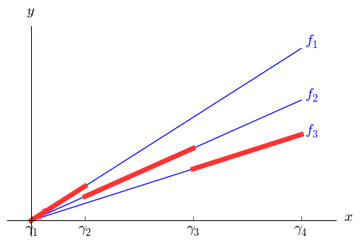
Let $y$ be a quantity (typically cost) that we wish to minimize. As before, we will assume that $y$ is a piecewise linear function of some variable $x$; for simplicity, I'll assume bounds $0 \le x \le U$ and $y\ge 0$. Let $0 = \gamma_1 < \cdots < \gamma_N < \gamma_{N+1}=U$ denote the breakpoints, and let $y=f_i(x)=\alpha_i x + \beta_i$ when $\gamma_i \le x < \gamma_{i+1}$, with the adjustment that the last interval is closed on the right ($f(U)=\alpha_N U + \beta_N$). With all units discounts, it is typical that the intercepts are all zero ($\beta_1 = \cdots = \beta_N = 0$) and cost ($y$) is proportional to volume ($x$), as seen in the first graph below, but we need not assume that. The second graph illustrates a somewhat more general case. In fact, we need not assume an economy of scale; the same modeling approach will work with a diseconomy of scale.

To model the discount, we need to know into which interval $x$ falls. Accordingly, we introduce binary variables $z_1,\ldots ,z_N$ and add the constraint $$\sum_{i=1}^N z_i = 1,$$ effectively making $\{z_1,\ldots , z_n\}$ an SOS1 set. Let $$M_i = \max_{0 \le x \le U} f_i(x)$$ for $i=1,\ldots,N$. Typically $M_i = f_i(U)$, but again we need not assume that. To connect the binary variables to $x$, we add for each $i\in \{1,\ldots,N\}$ the constraint $$\gamma_i z_i \le x \le \gamma_{i+1} z_i + U(1-z_i).$$ This just repeats the domain $0\le x \le U$ for all but the one index $i$ with $z_i = 1$; for that index, we get $\gamma_i \le x \le \gamma_{i+1}$.
The last piece is to relate the binary variables to $y$. We handle that by adding for each $i\in \{1,\ldots,N\}$ the constraint $$y\ge \alpha_i x + \beta_i - M_i(1-z_i).$$ For all but one index $i$ the right hand side reduces to $f_i(x)-M_i \le 0$. For the index $i$ corresponding to the interval containing $x$, we have $y\ge f_i(x)$. Since $y$ is being minimized, the solver will automatically set $y=f_i(x)$.
Adjustments for nonzero lower bounds for $x$ and $y$ are easy and left to the reader as an exercise. One last thing to note is that, while we can talk about semi-open intervals for $x$, in practice mathematical programs abhor regions that are not closed. If $x=\gamma_{i+1}$, then the solver has a choice between $z_i=1$ and $z_{i+1}=1$ and will choose whichever one gives the smaller value of $y$. This is consistent with typical all units discounts, where hitting a breakpoint exactly qualifies you for the lower price. If your particular problem requires that you pay the higher cost when you are sitting on a breakpoint, the model will break down. Unless you are willing to tolerate small gaps in the domain of $x$ (so that, for instance, the semi-open interval $[\gamma_i ,\gamma_{i+1})$ becomes $[\gamma_i , \gamma_{i+1}-\epsilon]$ and $x$ cannot fall in $(\gamma_{i+1}-\epsilon,\gamma_{i+1})$), you will have trouble modeling your problem.
Dear Paul,
ReplyDeleteIs there a reason you wouldn't use this technique to also model a continuous function? Moreover, if you wanted a concave piecewise linear (<=) constraint on a linear function L(x), could you define y as you have (without the minimization term in the objective) and then make the constraint: y <= f(x). I would think this would create a feasible region with the constraint L(x)>= f(x), correct? Would this only work if f(x) is concave? My first thought is it'd work for any piecewise linear function.
Also, would this method be slower than the SOS2 implementation?
Scott:
DeleteYou wouldn't use this technique for a continuous piecewise linear function if it had the correct convexity (convex if it's in the objective of a minimization problem or the left side of a $\le $ constraint, concave for maximization/$\ge $ constraint) because you wouldn't need it; you can handle those cases (previous post to this one) without introducing binary variables and branching.
If you need a constraint of the form $f(x)\le 0$ where $f$ is piecewise linear and concave (or $f(x)\ge 0$ where $f$ is convex), then the method described in this post works.
As to how this stacks up relative to SOS2, I'm not sure .. but I'm pretty sure it will depend on both the problem instance and the solver (because pretty much everything MIP-related depends on both). If you have really loose (inflated) values for the $M_i$, I think SOS2 will likely be faster. If you have fairly tight values for the $M_i$, I would not be surprised to find this method working better -- I think (but I'm not certain) that it will produce tighter bounds from the LP relaxations.
I hope that answered your questions.
Paul,
DeleteThank you for your reply. The only question I'm left with is this: Say I am minimizing a (different) linear function p(x). Can you enforce a piecewise linear constraint without adding a term to the objective function as you have done in this post?
My thought would be to use the method in this post, but then instead minimizing y, we add the additional constraint:
L(x) >=y
This way, I'd think that depending on the location of x, it would enforce the lower bound from the all units discount. My idea is that y is disconnected from the objective term and the search for an optimum will allow L(x) to push y all the way down to the piecewise linear constraint.
Thanks again!
Scott: Let's assume that $\underline{M}_{i}\le f_{i}(x)\le\overline{M}_{i}$ for all $i$ and for all $x\in\left[0,U\right]$. Let $\underline{M}^{*}=\min_{i}\underline{M}$ and $\overline{M}^{*}=\max_{i}\overline{M}$. What you want to do is add the constraints
Delete$$y\le f_{i}(x)+\left(\overline{M}^{*}-\underline{M}_{i}\right)\left(1-z_{i}\right)$$and$$y\ge f_{i}(x)-\left(\overline{M}_{i}-\underline{M}^{*}\right)\left(1-z_{i}\right).$$
Again, this is necessary only if $f$ is convex in a $\ge $ constraint or concave in a $le $ constraint (or if it appears in a $=$ constraint). For convex $f$ in a $\le $ constraint or concave $f$ in a $\ge $ constraint, you don't need the binary variables at all.
Oh! This way then you are in the interval it forces $y$ to equal $f_i (x)$, and then of course $y\leq L(x)$ enforces the correct constraint. Thank you very much, and thank you for running this blog-- it has been a very helpful resource for LP/IP/MILP techniques.
DeleteDear Paul,
ReplyDeleteI want to minimize a piecewise price function of multiple variables where the price is defined as a function of the total consumed quantity by many users and on different hours of the day. The price applied to each hour depends on the total consumption in that hour and is defined on successiv increasing intervals . The price get higher when we hit a breakpoint
The function to minimize is :
F = ∑ (P(h). Q(hi))
with Q(H) = Q(h1)+Q(h2)+ …+Q(hn) with H is some hour and N number of consumers .
I want to use binary variables z for every hour and apply the corresponding price in the constraints the same way you mentioned.
L(i)z(i) <= ∑ Q(hi) < U(i)z(i)
I am also using the 2 large constants M1 and M2 in my model.
∑ Q(hi) < U(i+1)z(i) + M1(1-z(i))
Y(h) >= (P(h). Q(hi)) - M2(1- z(i))
The objective function is rewritten as:
F = ∑ Y(h)
My question is how can I choose the appropriate values for the large constants M1 and M2 so that the optimization problem get solved (I am working with Matlab).
Right now my model is working but I am just trying with multiple values of M2 to get it work. And I am not sure at all about the values of M1.
Which other constraints or conditions should I take care of more to make this model return the minimum total cost.
Thank you very much.
Mohammed, I'm struggling a bit with your notation. so I'll have to give you a somewhat general answer.
DeleteYou do not need to use the same value of M1 across all constraints of the first type, nor the same value of M2 across all constraints of the second type. You want the tightest (smallest) possible value of each, consistent with the restriction that you must be sure not to turn a possible optimal solution infeasible by making the constraint too tight. If there is something in the model that says "total consumption in this particular hour cannot exceed a particular cutoff by a certain amount", for example, that "certain amount" might be a good value for M1 (or maybe M2? I'm a bit lost) for that specific hour.
Hi Paul,
ReplyDeleteThank you for the clarifications and for this very interesting blog.
I tried to enter correctly the mathematical formulas to explain the details but I didn't found a good mathematical online editor to author the formulas. I am sorry about this.
M1 is used in the constraint that specifies the upper limit in regard to the interval in which the total consumption ∑ Q(Ht) for a specific hour Ht may fall in. There is one such constraint for each possible interval and for each hour.
So, for Interval3 = (L3,U3) and hour h = (Ht), I will have this constraint for the upper limit :
∑ Q(Ht) < U3 . z3 + M1(1-z3) . While the constraint for the lower limit will be
L3 . z3 <= ∑ Q(Ht).
So I have : L3.z3 <= ∑ Q(Ht) < U3.z3 + M1(1-z3) to express the fact that ∑ Q(Ht) may fall in interval 3 by the branch and bound optimizer using the binary variables z.
M2 on the counterpart, is used in the constraints of the cost incurred for a specific hour. I will use M2 in the constraint of the total cost P(Ht) for a specific hour Ht for total consumption being in interval3:
Y(Ht) >= (P(Ht) * Q(Ht)) - M2 . (1- z3)
The objective function after variable substitution becomes:
F = ∑ Y(Ht) instead of
F = ∑ (P(Ht). Q(Ht)) which Ht = 1 .. 24.
Right now I am using only one value for M1 in all constraints and one value for M2 and I can see that M2 delivers the good results only after some threshold, while for M1 I was not able to see the effect of different values that I tested with.
Thank you.
For hour $H_t$, let $Q^*$ be a valid upper bound for $\sum Q(H_t)$. For interval 3, you can replace $M_1$ with $Q^* - U_3$, and more generally with $Q^*-U_k$ for interval $k$. Since $U_1 < U_2 < \dots$, this produces a decreasing sequence of $M_1$ values.
DeleteHi Paul,
DeleteThank you for the clarifications.
I feel more comfortable in using these formulas now.