Objective Constraints: The Sequel

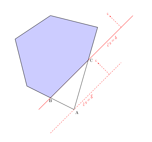
It belatedly occurred to me that I could have done a much better job explaining my previous post with a picture than I did with (copious) algebra. To recap the previous post, I claimed that adding a constraint to a mixed-integer programming model that puts an upper or lower bound on the objective value can cause solver performance to degrade of any of a several reasons, the least obvious of which is creating either dual degeneracy or multiple optimal solutions to the dual in the node linear program (LP) relaxation. We start with a model of the form\[ \begin{array}{lrclr} \mathrm{minimize} & c'x\\ \mathrm{s.t.} & Ax & \ge & b\\ & x & \ge & 0\\ & x_{i} & \in & \mathbb{Z} & (i\in I) \end{array} \](where $\mathbb{Z}$ is the set of integers), relax integrality and add a constraint $c'x\ge d$ to obtain the modified node LP\[ \begin{array}{lrclr} \mathrm{minimize} & c'x\\ \mathrm{s.t.} & Ax & \ge & b\\ & c'x & \ge & d\\ & x & \ge & 0. \end{array} \]The following picture depicts the scene at a typical node.

Vertex A represents the optimal solution in the absence of the added constraint (which runs through B and C), with optimal objective value $d^*$. As I mentioned in the previous post, at nodes where $d^*>d$ the added constraint will be nonbinding and just "extra baggage". Adding it can only benefit the user if $d>d^*$ at some nodes, as depicted here.

The shaded region is the feasible region including the objective constraint. The optimal value of the modified node LP is $d$, and B, C and every point on the line segment between them are all optimal solutions. So the node LP now has multiple optima, which will make the dual problem degenerate. The dual degeneracy can actually be seen in the picture. Slight increases or decreases in $d$ will shift the B-C edge up or down a bit, but that edge will clearly continue to be optimal. If we change $d$ to $d\pm \epsilon$ for small $\epsilon\gt 0$, the optimal objective value changes equally (to $d\pm \epsilon$), and so the dual variable $z$ corresponding to the objective constraint takes the value $z^*=1$.

Now observe what happens if we make small perturbations in the constraints that run through A and B or A and C. Either B or C will slide a bit in or out along the B-C edge (say, to B' or C' respectively), but the segment [B', C] or [B, C'] will continue to be optimal with the objective value $d$ unchanged. So the dual variables corresponding to those constraints must take value zero. Variables dual to the nonbinding constraints take value zero by virtue of the complementary slackness theorem of linear programming. We end up with all dual variables equal to zero except the one ($z$) connected to the added constraint. As I mentioned in the previous post, that is likely to have adverse consequences for pricing decisions, presolving, etc.

An upper bound constraint on the objective ($c'x\le d$) would switch the reduced feasible region to the triangle A-B-C, and A would be the sole optimum. This illustrates why the upper bound constraint is less likely to create algorithmic problems (other than drag). If it cuts through the feasible region (as depicted), it will be nonbinding, and the dual solution will be unaffected. If it misses the feasible region, the modified problem will be infeasible (and the node will be pruned). Only if the added constraint is tangent at A ($d=d^*$) do we run into misadventures.