Better Estimate, Worse Result

I thought I might use a few graphs to help explain an answer I posted on Quora recently. First, I'll repeat the question here:

In parametric optimization with unknown parameters, does a better estimator of the parameter always lead to better solutions to the actual problem?

Here we’re trying to minimize $f(x,\theta)$ with respect to $x$, but we don’t know the value of $\theta$. We may have several estimators of $\theta$, and we’re comparing them in a mean square error sense (or by some other loss function in general).

One would like to believe that better estimates lead to better answers, but the word "always" is a deal-breaker. Well, with one exception. The answer to the question is (trivially) yes if "better estimator" is interpreted to mean "estimator yielding better objective value". For mean square error or any other likely loss function, though, "better" is going to mean "closer to $\theta$" (in some sense of "closer"), and that's when things fall apart.

I'm going to take a couple of liberties in my answer. First, I'm going to change minimization of $f$ to maximization, just because it makes the pictures a little easier to interpret. Clearly that makes no meaningful difference. Second, I'm going to assume that maximization of $f$ is constrained. I can cobble together a similar but unconstrained counterexample by replacing the constraints with a penalty function (and assuming some bounds on the domain of $\theta$), but the constrained counterexample is (I think) easier to understand.

For my counterexample, I'll take a simple linear program in which the constraints are known with certainty but $\theta$ provides the objective coefficients:

$$\begin{array}{lrcl} \max & \theta_{x}x+\theta_{y}y\\ \text{s.t.} & x+y & \le & 3\\ & x & \le & 2\\ & y & \le & 2\\ & -x & \le & 0\\ & -y & \le & 0 \end{array}$$
I deliberately wrote the sign constraints $x \ge 0, y \ge 0$ "backwards" to fit Figure 1 below.

Figure 1

The feasible region is the polytope with vertices A, B, C, D and E. The dotted lines are (unit length) normals to the constraint hyperplanes. So $a^{(2)}$ is the coefficient vector (1, 1) of the first constraint, scaled to unit length, $a^{(5)}=(-1, 0)$ is the coefficient vector of the sign restriction on $x$ and so on. (I numbered the normals in clockwise order around the polytope, rather than in the order the constraints are written above.)

The red dashed vector represents a possible realization of the parameter $\theta$. Since we're maximize, $f$ increases in the direction that $\theta$ points, so for this particular realization vertex B is the unique optimum.

Note that $\theta$ in Figure 1 is between $a^{(1)}$ and $a^{2}$. This is not a coincidence. If $\theta$ is parallel to one of the constraint normals $a^{(j)}$, all points on the edge corresponding to that constraint will be optimal. If $\theta$ lies strictly between two constraint normals, the vertex where their edges intersect will be the unique optimum. This is easy to prove (but I won't bother proving it here).

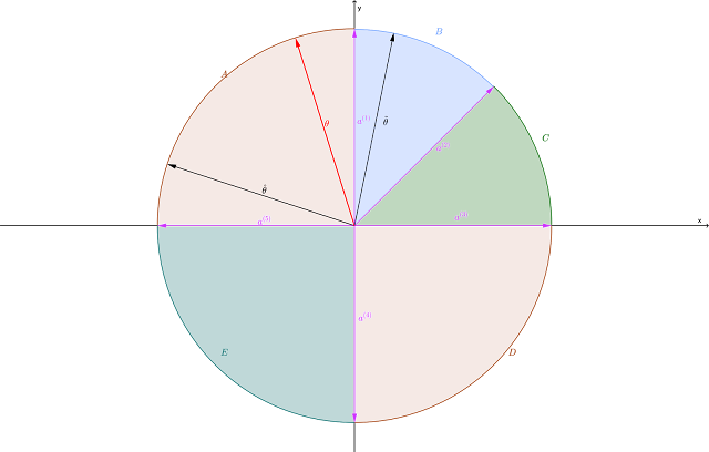
Figure 2 shows this situation in the same two dimensional space. The five constraint normals divide the space into five circular cones, with each cone corresponding to a vertex. If $\theta$ lands in the interior of a cone, that vertex is optimal. If it falls on an edge between two cones, both the corresponding vertices (and all points along the edge between them) are optimal.

Figure 2

In Figure 2 I've drawn a particular realization of $\theta$ (deliberately not the one from Figure 1), and two estimators $\hat{\theta}$ and $\tilde{\theta}$. Unfortunately, I'm limited to raster image formats and not vector formats in the blog, so the plots get rather fuzzy if you zoom on them. You'll have to take my word for it that $\hat{\theta}$ is the black vector just above the negative $x$ axis and $\tilde{\theta}$ is the black vector just clockwise of the positive $y$ axis. Alternatively, you can click on the image and download it or open it. (The images have transparent backgrounds, so I recommend opening them in your browser, or some other application that will supply a background.)

By design, I've selected them so that $\tilde{\theta}$ is geometrically closer to $\theta$ than $\hat{\theta}$ is. That should make $\tilde{\theta}$ the better estimator of the two in terms of squared error, absolute deviation ($L_1$ error), etc. Unfortunately, using $\tilde{\theta}$ results in vertex B being the unique optimum. Using the true coefficient vector $\theta$, vertex A is optimal, and the seemingly inferior estimator $\hat{\theta}$ also falls in the cone where A is optimal.

Thus using the "inferior" estimator $\hat{\theta}$ gets you the correct answer, albeit with a somewhat incorrect prediction for the value of the objective function. Using the "superior" estimator $\tilde{\theta}$ gets you a flat-out suboptimal solution. In Figure 1, the incorrect solution B looks to be not too far (geometrically) from the correct solution A, but I could easily cook this example so that B is a long way from A, guaranteeing a massively incorrect result.

All that said, I would still gravitate to the more accurate estimator and not sweat the occasional pathological outcome. Sadly, though, there is once again no guarantee that doing the right thing leads to the best result.