Revisiting a Joint Clustering Problem

In a previous post, I described a genetic algorithm for a problem posted on OR Stack Exchange. The problem involved grouping users and servers so as to maximize the total quality of service to all users. Every user in a cluster is served by every server in the cluster, but servers in other clusters interfere to some degree with the user's service.

The person who posted that problem recently posted another variation on OR SE. The new version of the problem is nearly, but not quite, identical to the previous version. "Servers" are now termed "transmitters", but the problem remains clustering transmitters and users, with limits on how many transmitters (but not how many users) belong to each cluster, and with the same objective function. The new version may be slightly easier thanks to one new restriction.

The user must belong to a cluster that has the transmitter providing the highest weight for the given user.

Thus the assignment of a transmitter to a cluster immediately implies the assignment to that cluster of all users for whom the specified transmitter has highest weight. (I will assume that ties for highest weight either do not occur or are broken whimsically.)

I put together two different mixed-integer programming (MIP) models for the problem. Both are rather complicated, in part because the objective function needs to be linearized. They are too big to squeeze into a blog post, so I put them in a PDF file. The models differ in the use of binary variables to assign transmitters. In the first model, a binary variable $x_{t,t'}$ is 1 if transmitters $t$ and $t'$ belong to the same cluster. In the second, a binary variable $x_{t,c}$ is 1 if transmitter $t$ belongs to cluster $c$. I coded both models in Java and ran them (using CPLEX as the MIP solver) on a few test problems with dimensions similar to what the original post contained (20 transmitters, 60 users). The first model was consistently smaller in size than the second and produced tighter bounds within whatever time limit I gave CPLEX.

The OR SE question also mentioned heuristics, so I coded up a couple of reasonably obvious ones. The first is a greedy construction heuristic. It initially puts each transmitter in a separate cluster, then repeatedly merges the pair of clusters that either produces the best improvement in the overall objective function. If no further improvement is possible and there are still more clusters than the number allowed, it merges whichever pair does the least damage to the objective. In all cases, mergers occur only if the merged cluster is within the allowed size limit.

The second heuristic is a pairwise swap heuristic. Given the (presumably feasible) solution from the first heuristic, it considers all pairs of transmitters belong to different clusters and, for each pair, evaluates the objective impact of swapping the two transmitters and performs the swap if it is beneficial. Note that swapping preserves the sizes of both clusters, so there is no question whether it is feasible. The heuristic keeps looping through pairs of transmitters until it is unable to find a useful swap.

In my experiments, I used the best solution from the second heuristic to "hot start" the first MIP model. (I ran into some difficulties getting the second MIP model to accept it as a starting solution, and frankly was not motivated enough to bother investigating the issue.) The results from one computational test (20 transmitters, 60 users, maximum cluster size 5) are fairly representative of what I saw in other tests. The construction heuristic got a solution with objective value 26.98 in 0.1 seconds on my desktop PC. The improvement heuristic ran for about 0.25 seconds and improved the objective value to 29.05. Running the first (better) MIP model using CPLEX 20.1 with a 10 minute time limit, starting from that solution, CPLEX improved the objective value to 29.62 with a final upper bound around 31.18. So the heuristic solution, which was obtained very quickly, was within 7% of optimal based on the bound and within 2% of the last solution CPLEX got within the 10 minute time limit.

Two caveats apply here. First, I did a minimal amount of testing. Second, and possibly more important, I randomly generated the transmitter-user weights using a uniform distribution. Having weights that follow a different distribution might affect both heuristic and model performance.

The Java code for both heuristics and both MIP models can be downloaded from my repository. It requires a recent version of Java (14 or later) since it uses the Record class, and it of course requires CPLEX (unless you want to delete that part and just play with the heuristics), but has no other dependencies.

Installing Rcplex in RStudio

This is an update to a previous post ("Installing Rcplex and cplexAPI"). Rcplex is a interface from R to the CPLEX optimization solver. A recent release (it's now at version 0.3-5) has made installation and updating much easier (no hacking of installer code required), provided you configure your environment correctly.

I use the RStudio IDE for almost everything related to R, including updating packages. A recent list of packages waiting to be updated included Rcplex 0.3-4, but when I told RStudio to update them all it balked at Rcplex. The workaround is actually quite simple. What follows is how I got to work in Linux Mint, but the same steps should work with any Linux distribution and I assume can be modified to work on Windows or Mac OS.

1. Find where the CPLEX binary lives. In my case, the path was "/home/paul/<stuff>/CPLEX_Studio201/cplex/bin/x86-64_linux/cplex".
2. In a terminal, create an environment variable CPLEX_BIN containing that path (unless you already have one). This can be done using the export command, as in "export CPLEX_BIN=/home/paul/<stuff>/CPLEX_Studio201/cplex/bin/x86-64_linux/cplex". Note that what I am exporting includes the name of the executable (that last "cplex"), not just the path to it. (I goofed on my first try by just specifying the path.)
3. Now invoke RStudio from the terminal and do the package update (or installation if you are getting it for the first time) as normal.

If you are not an RStudio user, you can install or update the package manually from a terminal by issuing the same export command followed by "R CMD INSTALL <path to download>/Rcplex_0.3-5.tar.gz" (updating the version number as necessary).

This was much less painful than previous installations. Thanks to the developers for maintaining the package and updating the installation scripts!

Update (04/23/2023): A recent update to the base R package (to 4.3.0) forced me to reinstall Rcplex, and of course I ran into problems. The current version of Rcplex in CRAN is 0.3-6. I followed the steps described above, and the C compiler barfed up some messages about multiple definitions of things and exited with an error code. Luckily, in the course of searching for explanations of the errors and fixes I tripped over the development page for Rcplex, where I found version 0.3-7, which had been released just a few days ago. That version installed correctly. Big thanks to the developers for continuing to maintain it.

Normalization Constraints

There are occasions where one might consider adding a constraint to an optimization problem specifying that $\|x\| \sim \nu,$ where $x$ is the solution vector, $\nu$ is a positive constant (usually 1, but sometimes something else), the norm is whichever norm (1, 2, $\infty$) suits the modeler's fancy, and the relation $\sim$ is whichever of $\le,$ $=$ or $\ge$ fits the modeler's needs. I can think of two somewhat common reasons for a constraint like this.

The first is a situation where $x$ is free to scale up or down and the modeler is trying to avoid having the solver choose ridiculously large or ridiculously small values for $x.$ Commonly, this is to prevent the solver from exploiting rounding error. As an example, consider the two group discriminant problem with a linear discriminant function, in which your observations have dimension $k$ and you have two samples, one of observations that should receive a positive discriminant score and one of observations that should receive a negative discriminant score. Let $P$ be an $m_P \times k$ matrix containing the first sample and $N$ an $m_N \times k$ matrix containing the second sample. Your goal is to find a coefficient vector $x\in \mathbb{R}^k$ and scalar $x_0\in \mathbb{R}$ that maximize the number of indices $i$ for which $\sum_j P_{i,j} x_j + x_0 \ge \delta$ plus the number of indices $i$ for which $\sum_j N_{i,j} x_j + x_0 \le -\delta,$ where $\delta > 0$ is a cutoff for how small a discriminant score can be and still be counted as nonzero. There is an obvious formulation as a mixed integer program using binary indicator variables for correct v. incorrect scores.

From a "pure mathematics" perspective, scaling the coefficients of the discriminant function (including $x_0$) up or down by a constant positive factor does not change whether an observation gets a positive, negative or zero score, but unfortunately the computer's finite precision arithmetic drags us out of the realm of "pure mathematics". Absent some sort of normalization, the solver might scale the coefficients way up to exploit some lucky rounding error (where an observation in the positive sample whose score should be zero or even negative gets a tiny positive score courtesy of rounding error, which becomes big enough to clear the $\delta$ threshold after the solution is scaled up). A normalization constraint is one way to avoid this, but I suspect a better way is just to impose bounds on the variables, which avoids any nonlinearities introduced by the norm function. Note, though, that when the domain of the variables contains both positive and negative values (true in the discriminant example, where coefficients can have either sign), bounds will not stop the solver from scaling the solution downward. If the solver wants to make the solution artificially small (for instance, if there is a penalty for scores that are incorrect by more than a particular amount), bounds will not prevent it; you will need a norm constraint.

The other situation I have encountered is one where zero is a feasible solution that is perhaps attractive from the perspective of the objective function but needs to be eliminated. An example of this recently popped up on OR Stack Exchange. Given a matrix $W,$ the author wants to find a vector $x\in\mathbb{R}^n$ that maximizes the number of nonnegative components of $Wx.$ The author turns this into a MIP model using binary indicator variables for whether a component is nonnegative or not. The catch here is that $x=0\implies Wx=0,$ so the zero solution trivially maximizes the objective (all components nonnegative). The author rules this out by adding the normalization constraint $\| x \|_1=n.$ The one-norm will introduce binary variables, either directly or indirectly (meaning they might be added internally by the solver).

For this situation, there is an alternative way to rule out zero. Suppose that we draw an observation $r\in\mathbb{R}^n$ from a continuous distribution over a set of full dimension. For simplicity, I like the uniform distribution, so I might take $r\sim U([-1, 1]^n).$ I would normalize the vector (changing $r$ to $r/\|r\|_2$) just to avoid the possibility that it is too close to a zero vector (or, if using a larger domain, too big). In lieu of the norm constraint, I would add the linear constraint $r^\prime x = 1.$ Clearly this eliminates $x=0,$ but does it eliminate other values of $x?$ Most likely not. If $r^\prime x \neq 0$ and if $x$ is free to scale, than the solver can scale an otherwise optimal $x$ to satisfy $r^\prime x = 1.$ Because $r$ is drawn from a continuous distribution over a full-dimensional domain, $\Pr(r^\prime x = 0)=0$ for any nonzero $x.$ So the only real concern would be if the optimal $x$ had a (nonzero) inner product with $r$ small enough that attempting to scale it to meet the normalization constraint would violate some bounds on the components of $x.$ That is a risk I'm usually willing to take.

Here is the punch line (and the motivation for this post). I suggested using the random product in lieu of the norm constraint in an answer I posted on OR SE. The author of the question commented that he had tried it, and it "improves performance by at least an order of magnitude". Presumably this is be eliminating the (explicit or implicit) binary variables in the computation of the 1-norm, along with an auxiliary variables and constraints used to implement the norm restriction.

I tested a genetic algorithm versus the author's MIP model (modified to replace the norm constraint with a random normalization) using CPLEX. If anyone is curious how the GA does, you can play with my R code (which, as usual, requires one library for the GA and a gaggle of libraries to use CPLEX).

A Heuristic Surprise

The maximum cut problem is one of those combinatorics problems that are deceptively easy to articulate and yet NP-annoying to solve. Given an undirected graph $G=(V,E)$, find a partition of $V$ into disjoint subsets $A$ and $B$ such that the set of edges in $E$ with one endpoint in $A$ and the other in $B$ (the "cut set") is as large as is possible. There is also a weighted version, where you maximize the total weights of the cut set rather than its cardinality.

Someone asked on OR Stack Exchange about a variant of the problem, in which there is a specified size (which the author called a "budget") for one of the sets, i.e., a constraint $|A|=b$ for some given $b$. This generated various suggestions, including some heuristics. I had a couple of thoughts about possible heuristics, and in playing with some computational examples found myself rather surprised by the results.

Mixed Integer Program

It is of course quite straightforward to write an integer or mixed-integer linear program for the problem. I'll assume that $V=\lbrace 1,\dots,N\rbrace$ and that $2\le b \le N-1$. Let variable $x_i$ be 1 if vertex $i\in V$ is in $A$ and 0 if it is in $B$, and let variable $y_{i,j}$ be 1 if edge $(i,j)\in E$ is in the cut set ($i\in A$ and $j\in B$ or vice versa) and 0 if not ($i$ and $j$ both in $A$ or both in $B$).

 

Please allow me a slight digression here. The $y$ variables can be declared either continuous or binary. The combination of objective and constraints will force the values to 0 or 1 even if they are declared as continuous. Force of habit, dating back to when I was using very early generation software on not particularly powerful (by current standards) computers, has me declaring every variable as continuous unless it has to be integer. On the other hand, it has been suggested to me that declaring such variables integer-valued may help solvers tighten bounds or fix variables. That makes sense to me, but in this particular model I don't see anything that would suggest making $y$ integer would help the solver.

Digression over, we can write the MIP model as

\begin{alignat*}{1} \max\sum_{(i,j)\in E}y_{ij}\\ \textrm{s.t. }\sum_{i\in V}x_{i} & =b\\ y_{ij} & \le x_{i}+x_{j}\quad\forall(i,j)\in E\\ y_{ij} & \le2-x_{i}-x_{j}\quad\forall(i,j)\in E\\ x_{i} & \in\left\{ 0,1\right\} \quad\forall i\in V\\ y_{ij} & \in\left[0,1\right]\quad\forall(i,j)\in E. \end{alignat*}

 

The first constraint enforces the "budget", while the second and third constraints ensure that $y_{ij}=0$ if $i$ and $j$ are on the same side of the partition. The objective function will force $y_{ij}=1$ if $i$ and $j$ are on different sides. The MIP model is easy to solve for small instances and grows more difficult as the number of vertices and the number of edges grows, and as $b$ gets closer to $N/2$ (since the number of possible partitions satisfying the budget increases).

Genetic Algorithm

Since the max cut problem is NP-hard, I suspect the budgeted version also is, and in any case it is likely that solving the MIP to optimality can take too long (or too much memory) in many cases. That led me to thinking about heuristics. One easy heuristic is to solve the MIP model but not to optimality, stopping at some arbitrary time or memory/node limit. That requires a MIP solver. Another possibility (among many) is a genetic algorithm.

I was fooling around with the problem in R, which has a very handy genetic algorithm library (named, rather suggestively, GA). Among other things, the GA library allows you to use a permutation as a "chromosome" (solution encoding). So we can define a candidate solution to be a permutation of $1,\dots,N$, and it's "fitness" is then the size of the cut set defined by setting $A$ equal to the first $b$ elements of the permutation.

Pairwise Swap

Another possibility that I suggested on OR SE was a simple pairwise swapping heuristic. Start by generating a random choice of $A$ (and, by implication, $B$) and calculate the size of the cut set. Now consider all pairs of vertices $i\in A$ and $j\in B$ and, for each pair, see what happens if you swap them (moving $i$ to $B$ and $j$ to $A$). If the size of the cut set increases, accept the swap; otherwise do not. This is a primitive example of a "neighborhood" search, and it can be used in fancier heuristics, including simulated annealing (where you occasionally accept a swap that actually makes the objective smaller, in order to get you out of your current neighborhood). To keep things simple, I suggested just doing pairwise swaps when the objective improved, with random restarts. That means assigning a time limit to the heuristic, and when you run out of acceptable swaps, start fresh with a new random solution until time is exhausted.

And the surprise is ...

I code the MIP model (solved with CPLEX), the GA and the swapping heuristic in R and ran them on a few random test cases, keeping dimensions small enough that CPLEX could solve the MIP reasonably quickly. Since the swapping heuristic relies on a time limit to stop it, I set a limit of two minutes. For the GA, I set a limit of 10,000 generations (which it never reached, as I expected) and a stagnation limit of 200 generations (meaning that, after 200 consecutive generations with no improvement in the best objective value, it would terminate). Early experiments suggested that the GA could stagnate pretty quickly, so I used an "island" GA (in which several smaller populations on "islands" evolve independently, with periodic migrations from one island to another to freshen the "genetic pools" on the islands).

My expectation was that the "sophisticated" GA would outperform the "primitive" swapping heuristic. Wrong! In the table below, I show the optimality gap (percent worse than the optimum, as computed by CPLEX) for the GA and the swap heuristic on six examples. Since the GA stagnates well before the two minute limit I gave to the swap heuristic, I also ran the GA with restarts (column "GA-R"), which restarted the GA with a new population each time it stagnated until the two minute limit was reached. The restarts improved the GA performance somewhat, but as you can see the swapping heuristic beat it on every one of the six test cases (and found the optimum in four out of six).

Graph			Gap
Nodes	Edges	Budget (b)	GA	GA-R	Swap
50	429	10	1.7%	1.7%	0.0%
50	490	20	3.0%	0.7%	0.0%
75	416	20	6.4%	4.3%	0.0%
75	416	30	6.8%	4.7%	0.4%
100	495	30	8.4%	7.8%	1.6%
100	990	25	9.1%	4.4%	0.0%

I don't expect the swapping heuristic to find the optimum this consistently on larger problems. Whether it would outperform the GA (with restarts) on tougher problems is an open question. Nonetheless, I take this as a reminder that sometimes simple heuristics can do a pretty good job.

My R notebook is available if you want to play with it. Fair warning: the notebook assumes you have CPLEX installed and loads seven R libraries (four for use with CPLEX, one for the GA, one to time execution of the heuristics and a separate one to set a time limit on the heuristics). If some of that does not interest you, you can of course edit out the related code and skip loading the corresponding libraries.

Smallest Polygon Containing A 2D Point Set

A question on OR Stack Exchange asked about an optimization model (specifically a MILP) for finding the "smallest hull" containing a finite set of points in the plane. The phrase "smallest hull" is rather fuzzy. In a follow up comment, the author of the question clarified that "smallest" means smallest area. That leaves the meaning of "hull". Note that any Hamiltonian path through the points would contain all the points (with all of them on its "boundary") and would have area zero. Based on a sample illustration added by the author, I will assume that "hull" here means polygon (but not necessarily a convex one).

I'm pretty sure that a MILP model could be devised, but I suspect it would be rather large and might solve slowly. So I looked at the possibility of a heuristic solution, and came up with something that seems to do pretty well but definitely does not produce an optimal solution in all cases. I got it working in R. You can see the full notebook (which includes the code) here. (Warning: It's almost 6MB, due to the presence of some graphs.) The notebook uses three R libraries: ggplot2 and plotly, for plotting; and interp, for generating a tesselation (more about that below). The plotly library is used just once, to generate an interactive plot with "tooltips" identifying each point, which is mainly useful for debugging. So if you don't feel like installing it, you can just delete any references to it and still run the important parts of the code.

Suppose we start with the following 2D point set.

Point set (with convex hull)

The heuristic first finds the convex hull of the points (shown above) and a Delaunay triangulation of them, using the tri.mesh function from the interp library. The triangulation is a collection of nonoverlapping triangles, with all vertices taken from the point set, such that no point is in the interior of any triangle. The next plot shows what the triangulation looks like.

Delaunay triangulation

The heuristic now takes a lap around the boundary of the convex hull. For each line segment $[a,b]$, it locates the (unique) triangle containing that edge. Let's say the third vertex of that triangle is $c$. If $c$ is not currently on the boundary, the heuristic adds it to the boundary, replacing the segment $[a,b]$ with the segments $[a,c]$ and $[c,b]$. It then deletes the $a-b-c$ triangle from the polygon, shaving off some area, and moves on to the next boundary segment.

This loop is repeated until a full circuit around the boundary fails to make any changes, at which point the heuristic terminates. Here is what the final polygon looks like.

Final polygon

What appear to be line segments sticking out in a few places are actually very skinny triangles. Clearly the heuristic did not select this polygon for its aesthetics.

The points were randomly generated in the unit square, which of course has area 1. For this example, the convex hull has area 0.865, while the final polygon has area 0.511, a reduction of almost 41%. At the same time, it is clear from the final plot that the solution is not optimal. There is one point left in the interior of the polygon, around $(0.493, 0.378)$. The heuristic cannot do anything about it because none of the triangles to which it belongs have an edge on the boundary. We could certainly add line segments from it to two boundary points, at $(0.483, 0.280)$ and $(0.450, 0.175)$, that currently share an edge. That would form a new triangle containing no other points, and we could drop the existing edge, adding the two new edges to boundary, and shed a little more area.

So the heuristic does not produce "nice looking" polygons, nor does it find an optimal solution, but my intuition after running a few examples is that it probably does reasonably well.

Worker Ordering

 A question ("Ordering of resources for maximizing success") on Mathematics Stack Exchange asks how to model the problem of sequencing workers under some unusual assumptions. You have 32 workers and 16 tasks. Each worker $i$ has a probability $w_i$ for success on any task. The probabilities vary by worker but not by task. Successes and failures are also assumed to be independent, meaning that if worker $i$ succeeds on one task, their probability of succeeding on the next task is still $w_i$, and if they fail on a task, the probability worker $i+1$ succeeds is still $w_{i+1}$. Once a worker fails, that worker is no longer available for any subsequent tasks. The objective is to order the workers so as to maximize the probability that all tasks are completed.

Answers posted on Math Stack Exchange asserted that sorting the workers into either ascending or descending probability order would be best. The question actually asked about how to model the decision problem, and I could not think of a good way to turn it into a tractable optimization model. So I decided to run a few experiments (in R) computing various permutations, with the thought that I would eventually land on a heuristic approach.

To my surprise, in every experiment I ran all permutations resulted in the same success probability. In other words, the answer to "what is the best order?" is "any order you like". I wrote out the explicit formula for success with three workers and two tasks, thinking I might see why the order did not matter, but derived no insights from it. So I was pretty much flummoxed.

Eventually, a retroactively obvious answer dawned on me. Suppose we put the workers in an arbitrary order, pad the list of tasks with dummy tasks (so there are essentially infinitely many tasks, the first 16 of which are real), and turn the workers loose sequentially until the last worker fails. Let $n_i$ be the number of successes for worker $i$. (Remember, $i$ stops after their first failure.) Since each attempt is an independent observation of a Bernoulli distribution with parameter $w_i$, $n_i$ has a geometric distribution with parameter $1-w_i$. As it turns out, the specific distribution does not matter to us. What matters is that, given our infinite supply of dummy tasks, the variables $n_1, \dots, n_{32}$ are independent of each other. Since the real tasks are at the front of our task queue, the probability of overall success is just $$\mathrm{Pr}\left(\sum_{i=1}^{32}n_{i}\ge16\right),$$which depends only on the sum, not the order of summation. So it becomes obvious that any ordering of the workers (and thus of the $n_i$ variables) yields the same likelihood of success.

If you want to see my R computations, they are in a notebook you can download.

Helping Babies

Before I get to what's on my mind, let me start by giving a shout out to the Resoundingly Human podcast from INFORMS. In each episode, host Ashley Kilgore interviews one or more OR academics or professionals about interesting recent work. Frequently, though not always, the subject matter pertains to a recent or forthcoming publication, but the discussions never get very technical, so they are suitable for a general audience. Episodes typical run in the vicinity of 15 to 20 minutes, which I find enough for a full exposition but not long enough to be tedious. They are generally quite well done.

What motivated me to post was the most recent episode, "Helping valuable donor milk reach infants in need", which I listened to while walking on a nature trail, feeding mosquitoes. The guest was Professor Lisa Maillart of the University of Pittsburgh, discussing a model she and colleagues developed to help donor milk banks convert donations into products for end use. If you are not familiar with milk banks (I actually was, not sure why), think "blood bank" but with donated breast milk replacing donated blood and babies in need replacing surgical patients in need. For greater detail, I recommend listing to the episode (linked above, approximately 20 minutes duration).

The application is the sort of thing that tends to give one warm fuzzy feelings. (Who doesn't like babies?) Moreover, during the podcast Prof. Maillart made a point that I think bears some reflection. I have not seen their model (the paper is not out yet), but from the sounds of it I think we can assume it is a production planning/blending model that likely resembles other models with which many of us are familiar. Early results from implementing the model seem to have produced substantial gains to the milk bank with which the authors collaborated. Prof. Maillart noted that, given the variety of constraints involved and the number of decisions to be made, scheduling production manually (based on experience, intuition or maybe just guesswork or subconscious heuristics) is challenging. In other words, for the non-OR person doing the planning, it is a "hard" problem, in part due to the number things to be juggled. To an OR person, it may not seem that hard at all.

For me, at least, "hard" means difficult to formulate because it involves some complicated constructs or some probabilistic/squishy elements, or difficult to formulate because something is nonlinear (and not easily approximated), or possibly difficult to solve because feasible solutions are in some way tough to find or the minimum possible scale (after decomposing or clustering or whatever it takes to get the dimensions down) still overwhelms the hardware and software.  (At this point I'll stop and confess that my perspective inevitably is that of an optimizer, as opposed to a simulator or a stochastic process <insert your own noun ending in "er" here -- I'm at a loss>.) For a typical person, going from five constraints of a particular sort (for instance, capacity limits on individual workers) to ten can be "hard". For an OR person, it just means the index range of a single constraint changes.

After listening to the episode, I am left wondering (not for the first time) how often people in the "real world" stare at "hard" problems that would seem relatively straightforward to an OR person ... if only we knew about them, which usually requires that the problem owner know about us. INFORMS is working to publicize both itself and the work of the OR community, but I think we still fly below almost everybody's radar.

Big-M versus Goals (Part II)

This is a continuation of my previous post, in which I discussed the common modeling issue of using a binary variable to enforce or relax a linear constraint. The standard approach to this uses what is commonly known as a "big M" constraint, but there are alternatives. The two that I mentioned in the previous post were a version of Benders decomposition frequently termed "combinatorial Benders cuts" (CBC) and an approach specific to CPLEX using disjunctive "goals". The previous post illustrated this using a mixed integer linear program (MILP) for the two-group discriminant problem.

I've used both "big M" and CBC before, but I had never used goals, and I was curious about the relative performance of the three methods. So I coded the discriminant problem from the previous post in Java (with a slightly different objective function, which is irrelevant to the discussion at hand) and ran the various models using four data sets that I have left over from a paper I wrote 30-ish years ago. The data sets relate to breast cancer (444+239), diabetes (500+268), liver disease (145+200) and (just to prove I don't have a morbid fascination with disease) radar returns (126+225). The numbers in parentheses are the sizes of the two samples.

I ran the problems using CPLEX 20.1 with a 10 minute time limit and default values for all parameters. For the CBC model, I used generic callbacks with a local copy of the LP subproblem for each thread (which will relate to memory use). The table below shows, for each combination of data set and model, the run time (in seconds), the final objective value (lower is better), the final bound (bigger is better) and the approximate peak memory use (in gigabytes, omitted for cases where the memory use was "trivial").

Data	Model	Time (s.)	Objective	Bound	Memory (GB)
Cancer	Big M	2.2	0.0124	0.0124	---
	CBC	6.5	0.0124	0.0124	---
	Goals	600	0.0124	0.0056	1.0
Diabetes	Big M	600	0.2057	0.0614	0.2
	CBC	600	0.3966	0.0598	2.9
	Goals	600	0.2239	0.0038	4.1
Liver	Big M	600	0.2521	0.1243	0.2
	CBC	600	0.3244	0.1013	7.6
	Goals	600	0.2639	0.0169	2.8
Radar	Big M	91	0.0190	0.0190	---
	CBC	139	0.0186	0.0186	0.2
	Goals	600	0.0190	0.0066	0.2

 

Before forging ahead, I'll note one small anomaly in the results for the radar data set. Both the "big M" and CBC methods got "provably optimal" solutions (lower bound = upper bound), but the CBC solution was slightly better (misclassifying six observations, versus seven for "big M"). I think this is just an issue with tolerance settings (constraint satisfaction tolerance, integrality tolerance or a combination of the two).

I've said on more than one occasion that the only valid generalization about integer programs is that there are no other valid generalizations about integer programs. That won't stop me from looking for possible patterns in the table, but it is important to keep in mind not only the small number of problems tried (four) and the specific nature (two-group discriminant analysis), but also the fact that I have fairly tight, data-based values of $M_i$ for the "big M" models. In two data sets, "big M" and CBC both got proven optimal solutions (with CBC being slower but not particularly slow). Both times, the goal approach also found an optimal solution (or optimal-ish in the radar case), but was nowhere getting the bound close to the optimal value. In the other two cases, goals did better on the primal side (found a better incumbent solution) but CBC did better on the dual side (found a tighter bound). Since CBC is busy hacking off infeasible candidate solutions and the goal approach is trying to satisfy goals, I suspect this pattern might generalize a bit.

On the two more difficult data sets (diabetes and liver disease), both CBC and goals used much more memory than "big M" did. In both cases, portions of the node file were being compressed and possibly shipped off to disk by CBC and goals, whereas "big M" never got to the point of consuming very much memory. I'll confess that I was expecting goals to be much more of a memory hog than CBC, since the goal "stack" gets replicated at every node, but CBC used much more memory than goals on the liver disease data set. Although I did not keep count, my guess is that indicates CBC was cranking out a huge number of Benders cuts. I think the memory use can be mitigated (somewhat) by making the cuts purgeable, but I did not bother to test that.

My last take-away: on the easy problems "big M" was fastest, and on the challenging problems "big M" had both the best incumbent value and the tightest bound. Again, this particular set of problems benefits from fairly tight $M_i$ values. So, henceforth, I will likely stick to "big M" whenever I think I have good values for $M$.

Big-M versus Goals

Much has been written (including by yours truly) about the trials and tribulations of "big M" integer programming models. A common use of "big M" is to let binary variables turn constraints on or off. So, for instance, $$a^\prime x \le b + Mz\quad (1)$$with $x$ a vector of continuous variables and $z$ a binary variable is intended to enforce $a^\prime x \le b$ when $z=0$ and not enforce it when $z=1$.

Large values of $M$ can contribute to weak relaxations (leading to slow progress on the bound), "leakage" (where a value of $z$ can be close enough to 0 that the solver considers it 0 to within rounding error while making $Mz$ big enough to relax the constraint), and various numerical problems. Small values of $M$ may make the constraint binding when it is supposed to be relaxed. Still, for most people the "big M" approach is the only way they know to model certain problem features.

One alternative, at least in some cases, is to use "combinatorial Benders decomposition" [1], in which the constraints in question are either enforced or ignored in a subproblem depending on the values of $z$ in the master problem. The good news is that this eliminates any worries about choosing $M$, since no coefficients $M$ are needed. The bad news is that (a) Benders decomposition is a bit advanced for many users, (b) it may require custom programming (as opposed to making the model in a high-level language and letting the modeling environment pass it to the solver), and (c) Benders decomposition is an "outer approximation", so the best bound may be a bit leisurely in converging to the optimum.

There is another alternative available, at least with CPLEX. Recent versions of CPLEX support "goals". The user's manual does a masterful job of not actually defining what a goal is -- according to the CPLEX 20.1 manual, goals are things that "allow you to take control of the branch & cut search procedure used by IBM ILOG CPLEX to solve MIP problems". Basically, a goal is an alternative form of a constraint (I think), which rather than explicitly appearing in the constraint matrix is put in a stack of goals, passed to nodes when they are created, and somehow used to influence the creation of child nodes (I think).

The tie-in to today's topic is that one type of goal provided by CPLEX is an "or" goal, which is what it sounds like: a disjunction of two or more constraints or goals. So an alternative to writing constraint (1) with the dreaded $M$ would be to use an "or" goal $$a^\prime x \le b \mathrm{\quad OR \quad} z=1.\quad (2)$$

I was curious about how well this would work, so I tried to do a comparison between "big-M" and goal-based models for a two-group discriminant problem. The gist of the model is as follows. We have as data a sample of vectors $x_i\in \mathbb{R}^n$ from two groups. Let $G_0$ and $G_1$ denote the indices belong to the first and second groups respectively. We want to find coefficients $w\in \mathbb{R}^n$, $w_0 \in \mathbb{R}$ for a linear function $f(x) = w^\prime x + w_0$ such that $f(x) \lt 0$ predicts membership of $x$ in the first group and $f(x) \gt 0$ predicts membership in the second group.

The specific model I started with (from some research I did in my much younger days) includes one more variable $d\ge \delta$ (where $\delta$ is some small positive constant) and binary variables $z_i$ signaling whether an observation is correctly ($z_i =0$) or incorrectly ($z_i=1$) classified. Variable $d$ captures the minimum absolute score of a correctly classified observation, which in essence represents the amount of separation between (correct) scores for the two groups. If $d$ is too small, you may end up classifying observations positive or negative based on what amounts to rounding error, hence the lower bound on $d$.

The "big M" version is as follows: $$\begin{align*} \min\quad\sum_{i}z_{i}-\epsilon d\\ \mathrm{s.t.}\quad w^{\prime}x_{i}+w_{0}+d & \le\phantom{-}M_{i}z_{i}\quad i\in G_{0}\\ w^{\prime}x_{i}+w_{0}-d & \ge-M_{i}z_{i}\quad i\in G_{1}\\ -1\le w & \le1\\ w_{0} & \quad \mathrm{free}\\ d & \ge\delta\\ z_{i} & \in\left\{ 0,1\right\} \quad\forall i. \end{align*}$$The model minimizes the number of misclassifications with a secondary criterion of maximizing separation. The coefficient $\epsilon$ is chosen to keep the objective contribution small enough that the solver is not tempted to make unnecessary misclassifications just to boost the value of $d$. Putting bounds on $w$ prevents huge coefficients for the classifier (which again could result in decisions being made based on rounding error). The model has been shown to work correctly.

The goal version of the model keeps the bounds on the variables and objective function but replaces all the "big-M" constraints with disjunctions of the form $w^\prime x_i +w_0 +d \le 0$ or $z_i=1$ for $i\in G_0$ and similarly for $i\in G_1$. In other words, "classify this observation correctly or pay the price for misclassifying it". I coded both models in Java and ran a test case, expecting both to produce an optimal classifier but unsure which would be faster. There was an unpleasant surprise waiting for me: CPLEX declared the goal-based model unbounded! It was right. You can satisfy all the disjunctions by declaring all the observations misclassified ($z_i = 1$ for all $i$). That lets you choose an arbitrarily large value for $d$, large enough that $\epsilon d$ is arbitrarily bigger than the sum of the $z$ variables, making the objective arbitrarily negative.

This is not a problem with the "big M" model, because no matter how large you make $M_i$, you still have a finite bound on the left side of each constraint. The fix was to come up with a defensible upper bound for $d$ and add it to the goal model, making the goal model bounded. With that fix in place, both models arrived at optimal solutions, in what was comparable time for the one test case I have run so far.

So the takeaway here is that if you want to use disjunctions to avoid "big M", you may need to take extra care to ensure that your model is bounded.

[1] Codato, G. and Fischetti, M. Combinatorial Benders' Cuts for Mixed-Integer Linear Programming. Operations Research 54(4), 2006, 756-766.

Vertex Numbering via GA

A question on OR Stack Exchange asks how to number vertices in a layered graph so that the endpoints of edges have similar numbers. Note that "numbering" the vertices here means numbering within layers (so that, for instance, every layer has a vertex numbered 1). We will assume that every node has a unique ID before we launch into the numbering process. The author of the question chose the sum of squared differences of endpoint labels for all edges as the objective function to minimize. The following image shows an example of a layered graph with a (probably suboptimal) numbering scheme. The numbers on the edges are their contributions to the objective function.

The prolific Rob Pratt noted that the problem can be modeled as an assignment problem with a quadratic objective function, using binary variables. That model produces an exact solution, given sufficient time and memory.

Note that numbering the nodes within a layer is equivalent to picking one of the possible permutations of the node IDs. The author of the question indicated receptiveness to a metaheuristic, so I decided to try coding a random key genetic algorithm (RKGA) for the problem. I've mentioned RKGAs before (for instance, here and here). As I understand it, they were originally designed for sequencing / scheduling problems, where things need to be permuted optimally, so an RKGA seemed like a natural choice. I coded both the integer programming (IP) model and the RKGA in Java, using CPLEX 20.1 as the IP solver and Watchmaker Framework 0.7.1 for the GA. The Watchmaker Framework has not been under active development for quite a few years, but it works well.

To use an RKGA, you need to come up with a coding for a "chromosome" (candidate solution) and a mechanism for decoding the chromosome into a solution to the original problem (in this case separate vertex permutations for each graph layer) such that the decoded chromosome is always feasible. I chose as my chromosome representation a double-precision vector with elements between 0 and 1, having one element per vertex in the original graph. Double-precision is probably overkill, but I'm in the habit of using double-precision rather than single-precision, so it was the path of least resistance. To decode the chromosome, I first had to chop it up into smaller vectors (one per layer) and then extract the sort index of each smaller vector. So, using the image above as an example, a chromosome would be a double vector with 2 + 5 + 3 = 10 components. If the last three components were (0.623, 0.021, 0.444) the sort indices would be (3, 1, 2), yielding the vertex numbering for the last layer in the image. To convert a double vector into a sort index vector, I used a Java library (ValueOrderedMap, described in this post) that I wrote some time back.

A GA can "stagnate", meaning cease to improve on the best known solution. One obvious reason for stagnation is that it cannot improve on an optimal solution, but stagnation can occur for other reasons. On small test problems, the GA tended to stagnate rather quickly, so I set a stagnation limit and put the GA in a loop that would restart it up to nine times or until a specified time limit (five minutes ... I wasn't very ambitious). On larger test problems, it was not as quick to stagnate, but it eventually did.

I used the GA's best solution as a starting solution for the IP model. On smaller test problems, CPLEX occasionally closed the gap to zero within five minutes but usually did not. On larger problems, CPLEX struggled to get the best bound above zero (100% gap) within five minutes. So I suspect the IP model is prone to loose bounds. An example of a "small" test problem is one with 29 vertices spread across five layers and 35 edges. (I worked mainly with sparse examples, to keep the size of the IP model down.)

Interestingly, in none of the trials did CPLEX improve on the initial solution provided by the GA. So it might be that the GA was consistently finding an optimum, although I cannot prove that. (On the few smaller instances where CPLEX reached provable optimality, the optimal solution was indeed the GA solution.) Note that, while the GA solution appeared optimal, that does not mean that each GA run produced an optimum. On the 29 vertex example mentioned above, CPLEX found a provable optimum with objective value 111. The GA ran 10 times (using about 92 seconds total), and of the 10 runs two stagnated at 111, five at 112, and three at 114. So even if the GA is prone to finding optimal solutions, it may require multiple starts to do so.

Smallest Pairwise Difference in R

 In a recent blog post, OR blogger Erwin Kalvelagen included some R code for a genetic algorithm, including an objective function that takes as input a vector $x\in\Re^n$ and returns the smallest absolute pairwise difference in its elements. The actual objective calls for the smallest difference in consecutive values, but Erwin correctly notes that the smallest absolute difference in any pair will automatically occur in consecutive values, so the "all pairs" approach yields the same objective value (and is considerably friendlier in the MIP and MINLP models he proposes).

I did a little experimenting and confirmed his opinion that the GA is unlikely to be competitive with the MIP model. That led me to a tangent involving the way the objective function for the GA is coded. Erwin used the obvious approach: two nested for loops to find all pairs of values once, avoiding comparing $x_i$ with $x_j$ and then (redundantly) $x_j$ with $x_i$, and avoiding comparing $x_i$ with itself. This approach does $O(n^2)$ work. An alternative approach is to first sort the vector $x$, which takes $O(n \log n)$ work, and then compute consecutive differences and their minimum value ($O(n)$). I put together a little R code to compare the two, and unsurprisingly the method with sorting is faster (and much faster when $n$ gets big).

There is another wrinkle to this. I've seen a number of articles and comments online asserting that explicit looping in R (as with Erwin's nested for loops) is inefficient, and should be avoided at all costs in favor of using vectorized functions (where the looping is presumably coded in C or C++ and baked into the compiled function). I've also seen contrary opinions saying that the concern about looping is overstated. There is also, I think, a middle ground: even if explicit loops are inefficient, that's likely only a concern if you are looping over very large objects, or looping many times, or both. Erwin's test case has $n=50$, which I suspect is not large enough to be worth worrying about the efficiency or inefficiency of looping (even though the GA will evaluate the objective function repeatedly).

So to test this, I cobbled together an R notebook (which you can find here) that tests all three versions of the objective function on vectors of various dimensions. As I thought, the sorted method dominates. Even at $n=50$ it's competitive with looping (although looping appears to be slightly faster), but at $n=2,000,000$ the sorting method takes about one third of a second on my PC (using R 4.1), whereas I estimate the nested loop method would take about 10 days (!).

The third method uses the (vectorized) outer product operator in R. It computes all $n^2$ absolute differences, whereas the nested loops calculate the $n(n-1)/2$ unique (nontrivial) differences, so in theory it does about twice the work the nested for loops do. Despite that, it is faster than the nested loops (though not nearly as fast as sorting). For $n$ around 5,000 to 10,000, the outer product approach seems to be about 10x faster than the nested loops.

So I take away two conclusions from this. The first is confirmation of a bit of wisdom that I believe I heard from Princeton computer scientist Robert Sedgewick in a MOOC based on his book (with Kevin Wayne) "Algorithms". Sorting is computationally cheap, so if you think it might help with a calculation, try it. The second is confirmation of the assertion that, even in the latest version (4.1) of R, explicit looping is probably slower, and quite possibly by a noticeable amount, than using vectorized methods ... when there are vectorized methods available.

If you are curious about the code for the alternative methods, it's embedded in the notebook.

 

Symmetric Difference of Sets in Java

The symmetric difference of two sets $A$ and $B$ is defined as $$C=(A \cup B)\backslash (A \cap B).$$It is the set of objects that belong to either $A$ or $B$ but not both. I've been working on some Java code for a research project in which I will need to compute the sizes of the symmetric differences of a large number of pairs of sets. The contents of the sets are nonnegative integers (Java type Integer), which makes life a bit simpler because integers are nicely ordered. (In Java-speak, Integer implements the Comparable<Integer> interface.) Since I will be doing a large number of differences, and since the sets involved will be moderately large (by my standards), I wanted to find the fastest way to compute a difference. So I wrote a Java program to generate random pairs of integer sets and compute the size of their symmetric difference four different ways.

Since the introduction of streams in Java (I believe in version 8), what I think is the most obvious/intuitive way to do it is to convert each set to a stream, filter out members of the other set, and count up the survivors. On the other hand, I am a happy user of the Apache Commons Collections library, whose CollectionsUtils class provides not one but two ways to do this. One is to use the subtract() method twice, switching the order of the arguments. This does the same thing that my first (stream-based) method does. The other is to use the disjunction() method, which calculates the symmetric difference in one invocation.

Equally obvious to me from a mathematical perspective, but not from a Java perspective, is to take the bitwise exclusive OR of the characteristic vectors of the two sets. Java contains a BitSet class, with set() and flip() methods for individual bits, which makes this easy to do.

My program runs the experiments on instances of both HashSet<Integer> and TreeSet<Integer>. Hash sets are generally faster, but tree sets have more features (and impose an internal ordering on their contents). My somewhat naive intuition was that having the contents accessed in ascending order would make differencing tree sets faster than differencing hash sets.

There are lots of moving parts here (how large the integers get, how big the sets involved in the comparisons are, ...), so I hesitate to read too much into the results. That said, here are some timing results using sets of cardinality between 100 and 200 with integers from 0 to 100,000. Times are in microseconds and are averages of 10,000 replications. (You can afford big samples when things go this quickly.)

Method	Streams	subtract()	disjunction()	BitSet
HashSet	10.07	36.40	62.15	9.68
TreeSet	23.79	35.37	60.94	7.21

 

I was surprised (OK, shocked) to find that the disjunction() method, which directly computes the symmetric difference, was almost twice as slow as two invocations of the subtract() method. Less surprising was that turning both sets into streams and filtering each other out was faster than calling subtract() twice. (Note that I am computing the size of the symmetric difference, not the symmetric difference itself. Uniting the two filtered streams or the two sets resulting from calls to subtract() into one combined set might move their times closer to those of disjunction()).

Another surprise to me was that the approach using streams was consistently slower with tree sets than it was with hash sets, despite the tree sets being inherently ordered. The characteristic vector (BitSet) approach seemed to have a slight preference for tree sets, but I'm not entirely sure that was consistent.

In this particular run, the characteristic vector approach (using BitSet) beat all comers. In other runs with similar parameters, streams sometimes beat BitSet and sometimes did not when the sets were instances of HashSet. With TreeSet, using BitSet appeared to be consistently faster. Let's contrast that with a second experiment, in which the integers are still between 0 and 100,000 but the sets are smaller (cardinality between 10 and 20).

Method	Streams	subtract()	disjunction()	BitSet
HashSet	3.18	5.96	9.75	6.24
TreeSet	3.11	4.89	8.10	4.07

 

Note that with the smaller sets the method using streams beats the characteristic vector (BitSet) method, and even the Commons Collections subtract() method may be a bit better than using the characteristic vector.

For my project, I am using instances of TreeSet, and I'm fairly certain the sets will (mostly) have cardinality in the low hundreds, so I will probably go with the BitSet approach. If anyone would like to run their own tests, my code is available in a GitLab repository.

Update: It belatedly occurred to me that in my research project, where I only need to get the size of the symmetric difference and not the symmetric difference itself, it might make sense to exploit the fact that the size of the symmetric difference between $A$ and $B$ is$$\vert A\vert + \vert B \vert - 2 \cdot \vert A \cap B\vert.$$So I can compute the size of the intersection, do a little arithmetic, and have the size of the symmetric difference.

I updated my code to include two versions of this approach. One version computes the intersection by streaming one set and filtering it based on inclusion in the other set. The other version uses the CollectionUtils.intersection() method. Once again, the CollectionUtils method was not competitive. Comparing the stream intersection method to the original stream approach and the characteristic vector approach using the original specifications for sets (cardinality 100 to 200), it seems the streamed intersection method is about twice as fast as the original stream method on both hash sets and tree sets (which makes sense, since it does with one stream what the original method did with two). It is also about twice as fast as the characteristic vector method on hash sets, but roughly half as fast on tree sets, as seen in the table below. (Times for the first two methods differ from previous tables because exact timings are unfortunately not reproducible.)

Method	Streams	BitSet	Intersection
HashSet	11.33	10.33	5.59
TreeSet	23.32	7.47	12.23

 

So the single stream intersection approach looks to be the fastest for computing the size (but, again, not contents) of the symmetric difference if I'm using hash sets, while the characteristic vector (BitSet) approach is fastest if I'm using tree sets.

A BDD with JGraphT

Decision diagrams, and in particular binary decision diagrams (BDDs) [1], were originally introduced in computer science to evaluate logic propositions or boolean functions. Lately, they've taken on multiple roles in discrete optimization [2]. I've been reading an excellent book [3] on them, with ideas about using BDDs in a current research project. As is my wont, I'll be coding the research in Java, so I wanted to do a little demo project to figure out how to build and process a BDD in Java.

Not wanting to reinvent any wheels, I looked for an open-source Java graph library with which to build the diagrams, and settled on JGraphT [4]. Not only does JGraphT have the necessary building blocks, it has much better online documentation than many libraries. Also, there is a very helpful article [5] about it on the Baeldung web site (which is itself an extremely useful site for all things Java).

A BDD is a directed, acyclic, layered multigraph with edge weights. If you're not familiar with the term "multigraph", it means that there can be two or more distinct edges between the same pair of nodes, in the same direction. In a BDD, each node represents a state of the system, with up to two outbound arcs, corresponding to true (1) or false (0) values for a particular decision variable. The decision variable is the same for all nodes in a particular layer. An arc is omitted if it represents a decision which, given the state, would make the solution infeasible. To keep the size of the BDD in check (somewhat), you do not want multiple nodes in a layer with the same state. The multigraph aspect arises because, in some circumstances, the next state may be the same regardless of the decision at the current node (so both arcs go to the same child node). Among the attractions of the JGraphT library are its support for nodes based on arbitrary classes (which in a BDD means the state at the node) and for multigraphs.

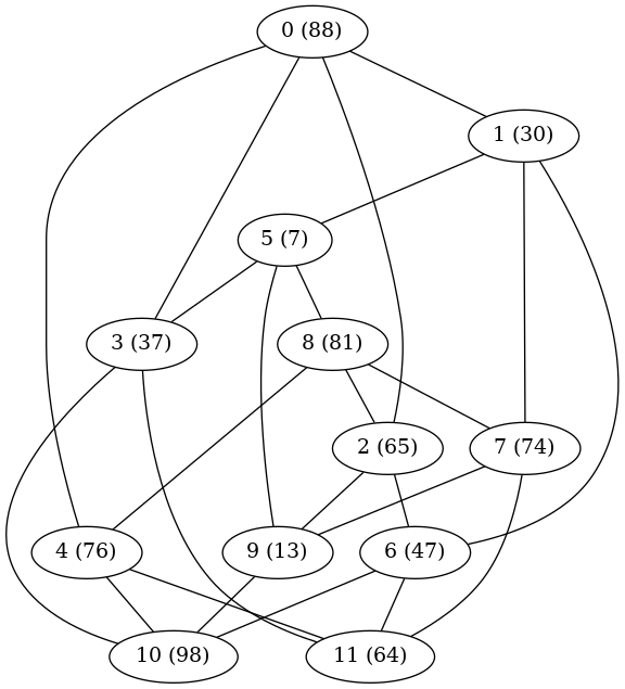
To learn how to build BDDs with JGraphT, I decided to solve a maximal independent set problem (MISP) [6] with integer node weights. This means choosing the subset of nodes with greatest total weight such that no two chosen nodes are adjacent. JGraphT contains routines to generate some well-known (to graph theorists -- less well known to me) graphs, and for convenience I chose the Chvátal graph [7], which has 12 nodes and 24 edges. Here is an illustration of the Chvátal graph, with the (randomly generated) node weights in parentheses.

My Java program uses routines in the JGraphT library to turn the graph into a DOT file [8], which it saves. I then use GraphViz [9] outside the Java program to convert the DOT file into the format I need for wherever the plot is going.

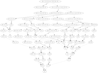
Using the same DOT export trick, I managed to generate a plot of the BDD, in which nodes display the set of vertices still available for addition to the independent set, arcs are solid if a vertex is being added to the independent and dotted if not, and solid arcs are annotated with the number of the vertex being added.

Unfortunately, Blogger does not accept SVG images and the BDD is a bit too big for a legible PNG graph. If you want to see a better image, click it and an SVG version should open in a new window or tab.

This post is already a bit long, so I won't go into details about the various coding issues I ran into or how I worked around them. I will point out one minor mathematical issue. Since the MISP is a maximization problem, the goal is to find the longest (in terms of weight, not number of edges) path from root node to terminal node in the BDD. JGraphT has a package containing shortest path algorithms, but no longest path algorithms. Fortunately, the number of layers in the graph is fixed (one layer per decision variable, plus one to hold the terminal node), which means the number $L$ of links in a longest path is fixed. So we simply find the maximum weight $W$ of any node in the graph, change the weight $w_e$ of each edge $e$ to $LW - w_e$, and find the shortest path using the modified weights. That path is guaranteed to be the longest path with respect to the original weights.

Last thing: As usual, my code is available for you to play with from my GitLab repository.

References

[1] Wikipedia entry: Binary decision diagram

[2] Decision Diagrams for Optimization (web page by Willem-Jan van Hoeve)

[3] Bergman, D.; Cire, A. A.; van Hoeve, W.-J. & Hooker, J. Decision Diagrams for Optimization. Springer International Publishing AG, 2016.

[4] JGraphT library

[5] Introduction to JGraphT (Baeldung)

[6] Wikipedia entry: Maximal independent set

[7] Wikipedia entry: Chvátal graph

[8] Wikipedia entry: DOT (graph description language)

[9] Graphviz - Graph Visualization Software

Lagrangean Relaxation: The Sequel

In a previous post, I looked at a way to solve a multiple assignment problem (where multiple users can be assigned to each server and each user can be assigned to multiple servers) using Lagrangean relaxation (LR). I won't repeat the details of the problem, or why LR was of interest, here. The post included some computational experiments in R, using CPLEX to get the optimal solution (for confirmatory purposes) and then trying out various nonlinear optimization algorithms on the Lagrangean function.

I've been looking for an open-source, derivative-free nonlinear optimizer (capable of taking box constraints) in Java, and I came across a couple in the Apache Commons Mathematics Library. Wanting to test one of them out, I repeated the experiment with the assignment problem in Java, again using CPLEX to get the optimal solution, and using the BOBYQA algorithm for minimizing the Lagrangean. As is my habit, I've made my Java code available via a GitLab repository for anyone who might want to see it. The Apache Commons library is a bit funky when it comes to using the optimization classes, so I had to do a little trial and error (and considerable staring at the Javadocs), along with a web search for examples. Hopefully my code is simple enough to be easy to digest.

A Math Puzzle as a Network

There is a standard type of math puzzle that has been around at least since I was a child. The details vary, but the concept is consistent. You are typically given a few initially empty containers of various (integer) capacities, an essentially infinite reservoir of something that goes in the containers, and a goal (integer) for how much of that something you want to end up with. You have to figure out how to reach the goal without having any measuring instruments, meaning that your operations are limited to emptying a container into the reservoir, filling a container from the reservoir, or moving content from one container to another until you empty the source or fill the destination, whichever happens first. (All this is done under the assumption of no spillage, meaning the originator of the puzzle did not have me in mind.) I think I've seen a variant that involves cutting things, where your ability to measure where to cut is limited to stacking pieces you already have as a guide to the piece you want to cut.

A question popped up on Mathematics Stack Exchange about how to solve one of these puzzles using dynamic programming (DP) with backward recursion. The problem at hand involves two jugs, of capacities seven and three liters respectively, and a lake, with the desired end state being possession of exactly five liters of water. The obvious (at least to me) state space for DP would be the volume of water in each jug, resulting in 32 possible states ($\lbrace 0,\dots,7\rbrace \times \lbrace 0,\dots,3 \rbrace$). Assuming the objective function is to reach the state $(5,0)$ with a minimal number of operations, the problem can be cast just as easily as a shortest path problem on a digraph, in which each node is a possible state of the system, each arc has weight 1, and arcs fall into one of the categories mentioned in the previous paragraph.

I was looking for an excuse to try out the igraph package for R, and this was it. In my R notebook, a node label "5|2" would indicate the state where the larger jug contains five liters and the smaller jug contains two. Arcs are labeled with one of the following: "EL" (empty the larger jug); "FL" (fill the larger jug); "ES" (empty the smaller jug); "FS" (fill the smaller jug); "PLS" (pour the larger jug into the smaller jug); or "PSL" (pour the smaller jug into the larger jug).

Assuming I did not screw up the digraph setup, a total of nine operations are required to get the job done. If you are interested, you can see my code (and the solution) in this R notebook.

A GA Model for a Joint Clustering Problem

A problem in grouping users and servers was posted on Mathematics Stack Exchange and OR Stack Exchange. (Someone remind me to rant about cross-posting in a future blog post. Just don't cross-post the reminder.) The gist of the problem is as follows. We have $S$ servers of some sort, and $U$ users. For each combination of user $u$ and server $s$, we have a parameter $h_{u,s}$ which pertains to the quality / strength / something of service user $u$ would get from server $s$. We are told to group users and servers into a predefined number $G$ of groups or clusters. Every user in cluster $g$ will be served by every server in cluster $g$, but servers in other clusters will interfere with the service to user $u$. (A possible application might be cellular phone service, where signals from towers to which you are not connected might interfere with your signal. Just guessing.)

There is one more parameter, the maximum number ($M$) of servers that can be assigned to a group. It is explicitly stated that there is no limit to the number of users that can be assigned to a group. I'm going to go a step further and assume that every group must contain at least one server but that there is no lower limit to the number of users assigned to a group. (If a group has no users, presumably the servers in that group get to relax and play video games or whatever.)

The objective is to maximize $\sum_{u=1}^U q_u$, the total quality of service, where $q_u$ is the quality of service for user $u$. What makes the problem a bit interesting is that $q_u$ is a nonlinear function of the allocation decisions. Specifically, if we let $\mathcal{S}_1, \dots, \mathcal{S}_G$ be the partition of the set $\mathcal{S} = \lbrace 1,\dots, S\rbrace$ of all servers, and if user $u$ is assigned to group $g$, then $$q_{u}=\frac{\sum_{s\in\mathcal{S}_{g}}h_{us}}{\sum_{s\notin\mathcal{S}_{g}}h_{us}}.$$Note that the service quality for user $u$ depends only on which servers are/are not in the same group with it; the assignments of other users do not influence the value of $q_u$.

 

An answer to the OR SE post explains how to model this as a mixed-integer linear program, including how to linearize the objective. That is the approach I would recommend. The original poster, however, specifically asked for a heuristic approach. I got curious and wrote a genetic algorithm for it, in R, using the GA library. Since this is a constrained problem, I used a random key GA formulation. I won't go into excessive detail here, but the gist is as follows. We focus on assigning servers to groups. Once we have a server assignment, we simply compute the $q_u$ value for each user and each possible group, and assign the user to the group that gives the highest $q_u$ value.

 

To assign servers to groups, we start with an "alphabet" consisting of the indices $1,\dots,S$ for the servers and $G$ dividers (which I will denote here as "|"). In the R code, I use NA for the dividers. A "chromosome" is an index vector that permutes the alphabet. Without loss of generality, we can assume that the first server goes in the first group, and the last divider must come after the last group, and thus we permute only the intervening elements of the alphabet. For instance, if $S=5$ and $G=3$, the alphabet is $1,2,3,4,5,|,|,|$ and a chromosome $(2, 7, 4, 6, 5, 3)$ would translate to the list $1, 2, |, 4, |, 5, 3, |$. (Each element of the chromosome is the index of an element in the alphabet.) I would interpret that as group 1 containing servers 1 and 2, group 2 containing server 4, and group 3 containing servers 3 and 5.

 

There is no guarantee that a random chromosome produces a server grouping that contains at least 1 and at most $M$ servers in every group, so we post-process it by going group by group and adjusting the dividers by the minimum amount necessary to make the current group legal. Once we have the servers grouped, we assign users by brute force and compute an overall fitness of the solution.

 

I am deliberately leaving out some (OK, many) gory details here. My R code and a test problem are contained in an R notebook that you are welcome to peruse. When I rerun the GA on the same test problem, I get different results, which is not surprising since the GA is a heuristic and is most definitely not guaranteed to produce an optimal solution. Whether the solution is "good enough", and whether it scales to the size problem the original poster has in mind, are open questions.

 

Restarting the MATE Panel

I know that Cinnamon is the trendy choice for desktop environment with Linux Mint,  but ever since an unfortunate misadventure with video drivers I have been using the somewhat more stable and somewhat faster MATE (pronounced Ma-Tay, per their home page) environment. Overall I am very happy with it. There are, however, occasional hiccups with the panel, the bar along one edge of the display (bottom in my case) containing launchers, tabs for open applications and general what-not. Occasionally, for reasons beyond me ken, some of the icons will be screwed up, duplicated, or duplicated and screwed-up. This morning, for instance, I found not one but three iterations of the audio output icon (looks like a loud speaker, used to set audio preferences). The first icon had the normal appearance, meaning audio was enabled, while the second and third were indicating that audio was muted. (Despite the 2-1 vote against, audio was in fact enabled.)

Glitches like that do not render the system unusable, but they are annoying. So I dug around a bit and discovered that the system command mate-panel. Run from a shell script or a launcher, the command mate-panel --replace seems to do the trick of restarting the panel (and hopefully fixing the glitch that made you restart it).  If you run the command from a terminal, be sure to push it to the background using an ampersand (mate-panel --replace &). Otherwise, it will tie up the terminal session, and when you break out of it (probably via Ctrl-C) the panel will rather unhelpfully evaporate.

Lagrangean Relaxation for an Assignment Problem

 A question on OR Stack Exchange asked about solving an assignment problem "heuristically but to optimality". The problem formulation (in which I stick as closely as possible to the notation in the original post, but substitute symbols for two numeric parameters) is as follows:

\begin{align*} \max_{d_{u,c}} & \sum_{u=1}^{U}\sum_{c=1}^{C}\omega_{u,c}d_{u,c}\\ \text{s.t. } & \sum_{c=1}^{C}d_{u,c}\le C_{\max}\ \forall u\in\left\{ 1,\dots,U\right\} \\ & \sum_{c=1}^{C}d_{u,c}\ge1\ \forall u\in\left\{ 1,\dots,U\right\} \\ & \sum_{u=1}^{U}d_{u,c}\le U_{\max}\ \forall c\in\left\{ 1,\dots,C\right\} \\ & d_{u,c}\in\left\{ 0,1\right\} \ \forall u,c. \end{align*} Here $d_{u,c}$ is a binary variable, representing assignment of "user" $u$ to "service provider" $c$, and everything else is a parameter. Each user must be assigned at least one provider and at most $C_\max$ providers, and each provider can be assigned at most $U_\max$ users. The objective maximizes the aggregate utility of the assignments.

One of the answers to the question asserts that the constraint matrix has the "integrality property", meaning that any basic feasible solution of the LP relaxation will have integer variable values. The recommended solution approach is therefore to solve the LP relaxation, and I agree with that recommendation. (I have not seen a proof that the matrix has the integrality property, but in my experiments the LP solution always was integer-valued.) That said, the author did ask about "heuristic" approaches, which got me wondering if there was a way to solve to optimality without solving an LP (and thus requiring access to an LP solver).

 I decided to try Lagrangean relaxation, and it seems to work. In theory, it should work: if the constraint matrix has the integrality property, and the LP relaxation automatically produces an optimal integer-valued solution, then there is no duality gap, so the solution to the Lagrangean problem should be optimal for the original problem. The uncertainty lies more in numerical issues stemming from the solving of the Lagrangean problem.

In what follows, I am going to reverse the middle constraint of the original problem (multiplying both sides by -1) so that all constraints are $\le$ and thus all dual multipliers are nonnegative. If we let $\lambda\ge 0$, $\mu\ge 0$ and $\nu\ge 0$ be the duals for the three sets of constraints, the Lagrangean relaxation is formulated as follows:

$$\min_{\lambda,\mu,\nu\ge0}LR(\lambda,\mu,\nu)=\\\max_{d\in\left\{ 0,1\right\} ^{U\times C}}\left(\sum_{u}\sum_{c}\omega_{u,c}d_{u,c}-\sum_{u}\lambda_{u}\left[\sum_{c}d_{u,c}-C_{\max}\right]\\+\sum_{u}\mu_{u}\left[\sum_{c}d_{u,c}-1\right]-\sum_{c}\nu_{c}\left[\sum_{u}d_{u,c}-U_{\max}\right]\right).$$

We can simplify that a bit:

$$\min_{\lambda,\mu,\nu\ge0}LR(\lambda,\mu,\nu)=\\\max_{d\in\left\{ 0,1\right\} ^{U\times C}}\left(\sum_{u}\sum_{c}\left[\omega_{u,c}-\lambda_{u}+\mu_{u}-\nu_{c}\right]d_{u,c}\\+C_{\max}\sum\lambda_{u}-\sum_{u}\mu_{u}+U_{\max}\sum_{c}\nu_{c}\right).$$

The inner maximization problem is solvable by inspection. Let $\rho_{u,c}= \omega_{u,c}-\lambda_{u}+\mu_{u}-\nu_{c}$. If $\rho_{u,c} > 0$, $d_{u,c}=1$. If $\rho_{u,c} < 0$, $d_{u,c}=0$. If $\rho_{u,c} = 0$, it does not matter (as far as the inner problem goes) what value we give $d_{u,c}$. So we can rewrite the outer (minimization) problem as follows:

$$\min_{\lambda, \mu, \nu \ge 0}LR(\lambda,\mu,\nu)=\\\sum_{u}\sum_{c}\left(\rho_{u,c}\right)^{+}+C_{\max}\sum\lambda_{u}-\sum_{u}\mu_{u}+U_{\max}\sum_{c}\nu_{c}.$$

$LR(\lambda,\mu,\nu)$ is a piecewise-linear function of its arguments, with directional gradients, but is not continuously differentiable. (Things get a bit tricky when you are on a boundary between linear segments, which corresponds to having $\rho_{u,c}=0$ for one or more combinations of $u$ and $c$.)

I coded a sample instance in R and tested both solving the LP relaxation (using CPLEX) and solving the Lagrangean problem, both using a derivative-based method (a version of the BFGS algorithm) and using a couple of derivative-free algorithms (versions of the Nelder-Mead and Hooke-Jeeves [1] algorithms). Importantly, all three algorithms are modified to allow box constraints, so that we can enforce the sign restriction on the multipliers.

You can download my code in the form of an R notebook, containing text, output and the code itself (which can be extracted). In addition to CPLEX, it uses a gaggle of R libraries: magrittr (for convenience); ompr, ompr.roi, ROI and ROI.plugin.cplex for building the LP model and interfacing with CPLEX; and dfoptim for the Nelder-Mead and Hooke-Jeeves algorithms. (The BFGS algorithm comes via the optim() method, part of the built-in stats library.) If you want to play with the code but do not have CPLEX or some of the libraries, you can just delete the lines that load the missing libraries along with the code that uses them.

Based on limited experimentation, I would say that Nelder-Mead did not work well enough to consider, and BFGS did well in some cases but produced somewhat suboptimal results in others. It may be that tweaking some control setting would have helped with the cases where BFGS ran into trouble. Hooke-Jeeves, again in limited testing, consistently matched the LP solution. So if I needed to come up with some hand-coded way to solve the problem without using libraries (and did not want to write my own simplex code), I would seriously consider using Hooke-Jeeves (which I believe is pretty easy to code) on the Lagrangean problem.

[1] Hooke, Robert and Jeeves, T. (1961) "Direct search'' solution of numerical and statistical problems. Journal of the ACM, Vol. 8, No. 2, 212-229.